Where in London does the Police Stop & Search most People?

Story of the visualisation
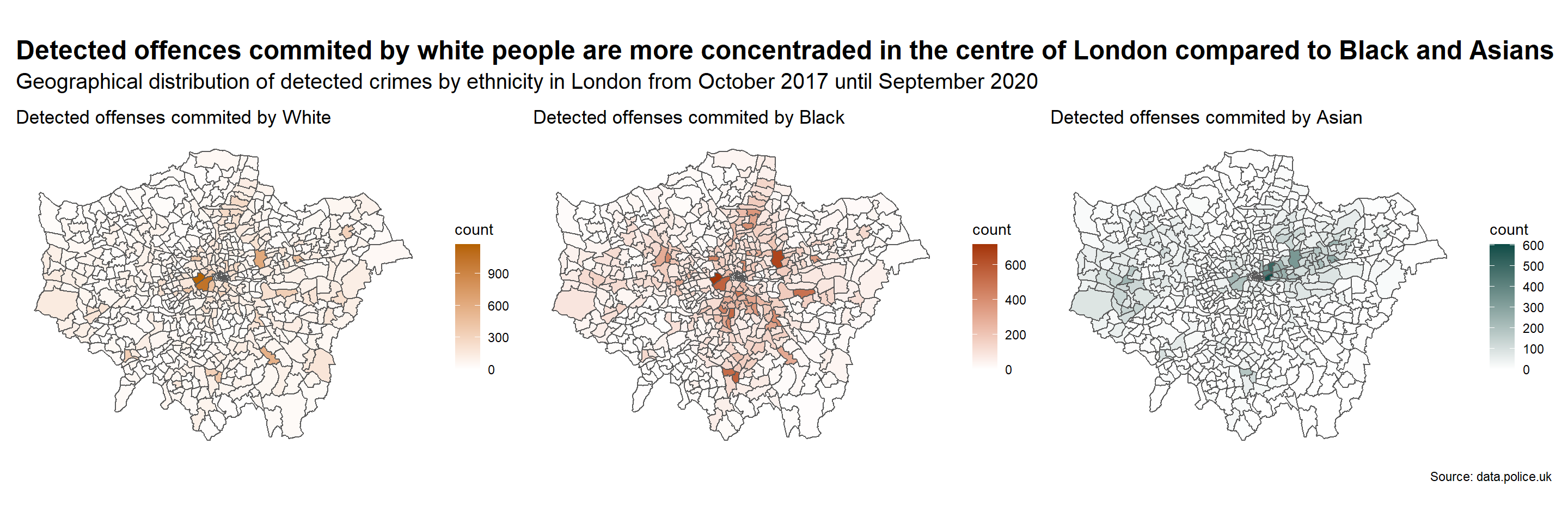
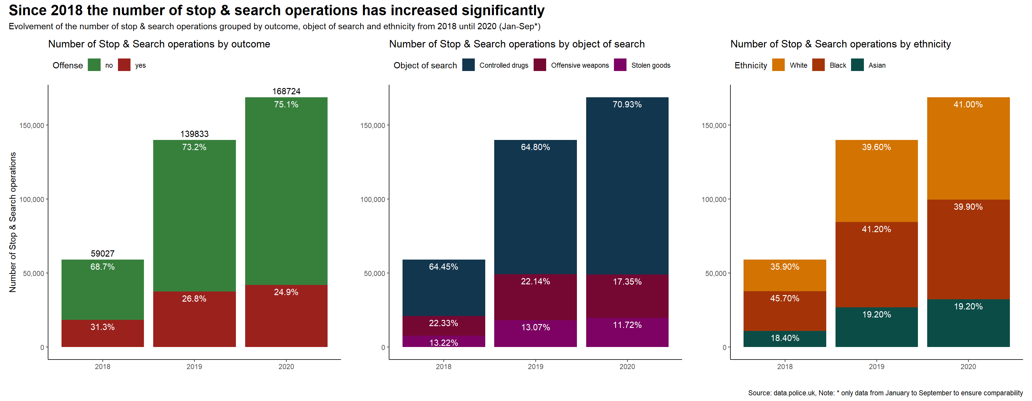
As starting point, I analysed changes in the number of Stop & Search operations and detected offenses over time from October 2017 until September 2020. While the plots showed a significant increase in the number of both over time, the percentage of detected offenses compared to the number of stop & search operations decreased from 31.3% to 24.9%. Furthermore, the distribution of objects of search and of ethnicity of the searched individuals did not change over time. Having detected this, I decided to not look at changes over time when it comes to these variables but rather at other variables. To analyse the geographical distribution of stop & search operations as well as of the detected offenses, I map the respective numbers for each ward. The distribution of searches and crimes is not homogeneous, but they preliminary happen in the centre of London. But, no significant difference between the distribution of stop & search operations and detected offenses can be seen. Therefore, in my further analysis I will focus solely on the geographical distribution of number of detected offenses. Finally, I plot the data on the map of London grouped by ethnicity and by object searched to detect patterns in the geographical distribution. From the created maps it is evident, that the detection of crimes related to offensive weapons is more geographically dispersed than related to drugs or stolen goods. Moreover, detected offences committed by white people are more concentrated in the centre of London compared to Black and Asians
Initial overview of the data
# Number of Stop & Search operations by gender
table1 <- stop_search_all %>%
  count(gender, sort=TRUE)
kbl(table1,col.names=c("Gender","Count")) %>%
kable_styling()| Gender | Count |
|---|---|
| Male | 636838 |
| Female | 45848 |
| NA | 9160 |
| Other | 385 |
# Number of Stop & Search operations by object of search
table2 <- stop_search_all %>%
  count(object_of_search, sort=TRUE)
kbl(table2,col.names=c("Object of search","Count")) %>%
kable_styling()| Object of search | Count |
|---|---|
| Controlled drugs | 418103 |
| Offensive weapons | 119754 |
| Stolen goods | 74515 |
| Evidence of offences under the Act | 32438 |
| Anything to threaten or harm anyone | 24843 |
| Articles for use in criminal damage | 14474 |
| Firearms | 4583 |
| NA | 1800 |
| Fireworks | 1721 |
# Number of Stop & Search operations by ethnicity
table3 <- stop_search_all %>%
  count(officer_defined_ethnicity, sort=TRUE)
kbl(table3,col.names=c("Ethnicity","Count")) %>%
kable_styling()| Ethnicity | Count |
|---|---|
| Black | 274058 |
| White | 257779 |
| Asian | 118568 |
| Other | 28232 |
| NA | 13594 |
# Number of Stop & Search operations by age
table4 <- stop_search_all %>%
  count(age_range)
kbl(table4,col.names=c("Age","Count")) %>%
kable_styling()| Age | Count |
|---|---|
| 10-17 | 116893 |
| 18-24 | 235540 |
| 25-34 | 144190 |
| over 34 | 104597 |
| under 10 | 126 |
| NA | 90885 |
#I read London Wards shapefile
london_wards_sf <- read_sf(here("data/London-wards-2018_ESRI/London_Ward.shp"))

# I control the type of geometry that the shapefile has
st_geometry(london_wards_sf)#Geometry is Polygon
## Geometry set for 657 features
## geometry type: POLYGON
## dimension: XY
## bbox: xmin: 504000 ymin: 156000 xmax: 562000 ymax: 201000
## projected CRS: OSGB 1936 / British National Grid
## First 5 geometries:# I transfrom CRS to 4326
london_wgs84 <- london_wards_sf %>%
st_transform(4326) # transfrom CRS to WGS84, latitude/longitude
london_wgs84$geometry## Geometry set for 657 features
## geometry type: POLYGON
## dimension: XY
## bbox: xmin: -0.51 ymin: 51.3 xmax: 0.334 ymax: 51.7
## geographic CRS: WGS 84
## First 5 geometries:Filter data
# concentrate in top three searches, age_ranges, and officer defined ethnicities
which_searches <- c("Controlled drugs", "Offensive weapons","Stolen goods" )
which_ages <- c("10-17", "18-24","25-34", "over 34")
which_ethnicity <- c("White", "Black", "Asian")

stop_search_top <- stop_search_all %>%

  #filter out rows with no latitude/longitude
  filter(!is.na(lng)) %>%
  filter(!is.na(lat)) %>%

  # concentrate in top searches, age_ranges, and officer defined ethnicities
  filter(object_of_search %in% which_searches) %>%
  filter(age_range %in% which_ages) %>%
  filter(officer_defined_ethnicity %in% which_ethnicity) %>%

  # I relevel factors so everything appears in correct order
  mutate(
    object_of_search = fct_relevel(object_of_search,
                                   c("Controlled drugs", "Offensive weapons","Stolen goods")),
    age_range = fct_relevel(age_range,
                            c( "10-17","18-24", "25-34", "over 34")),
    officer_defined_ethnicity = fct_relevel(officer_defined_ethnicity,
                                            c("White", "Black", "Asian")),
    offense= case_when(outcome %in% c("Nothing found - no further action", "A no further action disposal")~ "no",
    TRUE ~ "yes"
  ))
Development over time
p1 <- stop_search_top %>%
  filter(month %in% c(1,2,3,4,5,6,7,8,9)) %>%
  filter(year != 2017) %>%
  group_by(year, object_of_search) %>%
  summarise(count=n()) %>%
  mutate(percentage=((count/sum(count)))) %>%
  ggplot(aes(y=count, x=year, fill=object_of_search))+
  geom_col()+
  labs(y="", x="", title= "Number of Stop & Search operations by object of search", fill= "Object of search")+
  geom_text(aes(label=percent(round(percentage,4))),geom ='text', col = 'white', vjust=1.5, position= position_stack())+
  theme_classic()+
  scale_y_continuous(label=comma)+
  scale_fill_manual(values=c("#12364E", "#750833", "#7D0263"))+
  theme(legend.position='top',
        legend.justification='left',
        legend.direction='horizontal')+
  NULL

p2 <- stop_search_top %>%
  filter(month %in% c(1,2,3,4,5,6,7,8,9)) %>%
  filter(year != 2017) %>%
  group_by(year, officer_defined_ethnicity) %>%
  summarise(count=n()) %>%
  mutate(sum = sum(count), percentage=((count/sum))) %>%
  ggplot(aes(y=count, x=year, fill=officer_defined_ethnicity))+
  geom_col()+
  labs(y="", x="", title= "Number of Stop & Search operations by ethnicity", fill= "Ethnicity")+
  geom_text(aes(label=percent(round(percentage,3))),geom ='text', col = 'white',vjust=1.5, position= position_stack() )+
  theme_classic()+
  scale_y_continuous(label=comma)+
  scale_fill_manual(values=c("#D27302", "#A43407", "#0C4C47"))+
  theme(legend.position='top',
        legend.justification='left',
        legend.direction='horizontal')+
  NULL


p3 <- stop_search_top %>%
  filter(month %in% c(1,2,3,4,5,6,7,8,9)) %>%
  filter(year != 2017) %>%

  group_by(year, offense) %>%
  summarise(count=n()) %>%
  mutate(percentage=((count/sum(count)))) %>%
  ggplot(aes(y=count, x=year, fill=offense))+
  geom_col()+
  labs(y="Number of Stop & Search operations", x="", title= "Number of Stop & Search operations by outcome", fill= "Offense")+
  geom_text(aes(label=percent(round(percentage,4))),geom ='text', col = 'white',vjust=1.5, position= position_stack() )+
  theme_classic()+
  scale_y_continuous(label=comma)+
  geom_text(
    aes(label = stat(y), group = year),
    stat = 'summary', fun = sum, vjust = -0.5, col= "black")+
  scale_fill_manual(values=c("#37803C", "#9B211D"))+
  theme(legend.position='top',
        legend.justification='left',
        legend.direction='horizontal')+
  NULL

(p3 +p1 +p2) + plot_annotation(
  title = 'Since 2018 the number of stop & search operations has increased significantly',
  subtitle = 'Evolvement of the number of stop & search operations grouped by outcome, object of search and ethnicity from 2018 until 2020 (Jan-Sep*)',
  caption = 'Source: data.police.uk, Note: * only data from January to September to ensure comparability', theme = theme(plot.title = element_text(size = 18, face= "bold"))
)
Maps: Geographical distributions
# Here we retrieve and apply the CRS of london_wgs84
stop_search_sf <-  st_as_sf(stop_search_top,
                              coords=c('lng', 'lat'),
                              crs=st_crs(london_wgs84))

#glimpse(stop_search_sf) #now geometry added
# Count how many S&S happened inside each ward
london_all <- london_wgs84 %>%
mutate(count = lengths(
st_contains(london_wgs84,
stop_search_sf)))
p1 <- ggplot(data = london_all, aes(fill = count)) +
geom_sf() +
scale_fill_gradient(low = "white", high = "#37803C")+
theme_minimal()+
coord_sf(datum = NA) + #remove coordinates
labs(title = "Stop & Search Operations in London") +
theme(axis.text = element_blank()) +
theme(strip.text = element_text(color = "white"))+
NULL
# filter out stop-and-search where no further action was taken
offense_sf <- stop_search_sf %>%
filter(offense == "yes")
# Count how many offenses happened inside each ward
london_offense <- london_wgs84 %>%
mutate(count = lengths(
st_contains(london_wgs84,
offense_sf)))
p2 <- ggplot(data = london_offense, aes(fill = count)) +
geom_sf() +
scale_fill_gradient(low = "white", high = "#9B211D")+
theme_minimal()+
coord_sf(datum = NA) + #remove coordinates
labs(title = "Offense detected through Stop & Search Operation in London") +
theme(axis.text = element_blank(),
strip.text = element_text(color = "white")
)+
NULL
(p1 + p2) + plot_annotation(
title = 'Wards with more stop & search operations detect more offenses',
subtitle = 'Geographical distribution of search & stop operations and detected offenses from October 2017 until September 2020',
caption = 'Source: data.police.uk', theme = theme(plot.title = element_text(size = 18, face= "bold"), plot.subtitle = element_text(size = 15)))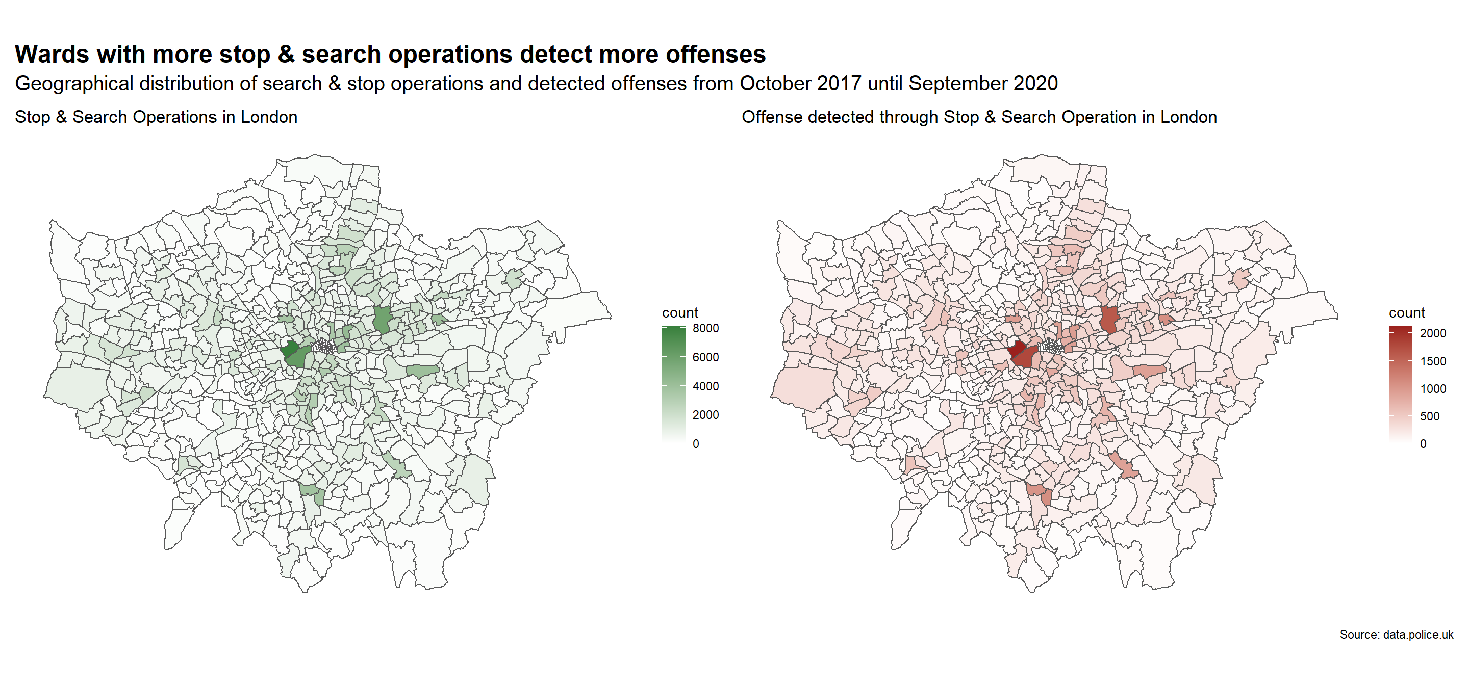
# filter out object of search 1
vis1a_sf <- offense_sf %>%
  filter(object_of_search== "Controlled drugs")

# Count how many S&S happened inside each ward
  london_vis1a <- london_wgs84 %>%
  mutate(count = lengths(
    st_contains(london_wgs84,
                vis1a_sf)))

p1 <- ggplot(data = london_vis1a, aes(fill = count)) +
   geom_sf() +
   scale_fill_gradient(low = "white", high = "#12364E", na.value = "transparent")+
  theme_minimal()+
  coord_sf(datum = NA) + #remove coordinates
  labs(title = "Detected offenses when searched for Controlled drugs") +
  theme(axis.text = element_blank(),
        strip.text = element_text(color = "white")
        )+
  NULL

# filter out object of search 2
  vis1b_sf <- offense_sf %>%
  filter(object_of_search== "Offensive weapons")

# Count how many S&S happened inside each ward
  london_vis1b <- london_wgs84 %>%
  mutate(count = lengths(
    st_contains(london_wgs84,
                vis1b_sf)))

p2 <- ggplot(data = london_vis1b, aes(fill = count)) +
   geom_sf() +
   scale_fill_gradient(low = "white", high = "#750833", na.value = "transparent")+
  theme_minimal()+
  coord_sf(datum = NA) + #remove coordinates
  labs(title = "Detected offenses when searched for Offensive weapons") +
  theme(axis.text = element_blank(),
        strip.text = element_text(color = "white")
        )+
  NULL

# filter out object of search 3
  vis1c_sf <- offense_sf %>%
  filter(object_of_search== "Stolen goods")

# Count how many S&S happened inside each ward
  london_vis1c <- london_wgs84 %>%
  mutate(count = lengths(
    st_contains(london_wgs84,
                vis1c_sf)))

p3 <- ggplot(data = london_vis1c, aes(fill = count)) +
   geom_sf() +
   scale_fill_gradient(low = "white", high = "#7D0263", na.value = "transparent")+
  theme_minimal()+
  coord_sf(datum = NA) + #remove coordinates
  labs(title = "Detected offenses when searched for Stolen goods") +
  theme(axis.text = element_blank(),
        strip.text = element_text(color = "white")
        )+
  NULL


(p1 + p2 +p3) + plot_annotation(
  title = 'Offensive weapons is a more geographically dispersed crime than controlled drugs and stolen goods',
  subtitle = 'Geographical distribution of detected crimes by object of search in London from October 2017 until September 2020',
  caption = 'Source: data.police.uk', theme = theme(plot.title = element_text(size = 18, face= "bold"), plot.subtitle = element_text(size = 15)))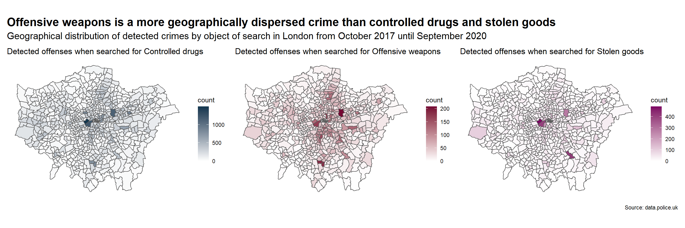
# filter out ethnicity 1
vis2a_sf <- offense_sf %>%
    filter(officer_defined_ethnicity== "White")

# Count how many S&S happened inside each ward
  london_vis2a <- london_wgs84 %>%
  mutate(count = lengths(
    st_contains(london_wgs84,
                vis2a_sf)))

p1 <- ggplot(data = london_vis2a, aes(fill = count)) +
   geom_sf() +
   scale_fill_gradient(low = "white", high = "#B56200", na.value = "transparent")+
  theme_minimal()+
  coord_sf(datum = NA) + #remove coordinates
  labs(title = "Detected offenses commited by White") +
  theme(axis.text = element_blank(),
        strip.text = element_text(color = "white")
        )+
  NULL

# filter out ethnicity 2
  vis2b_sf <- offense_sf %>%
    filter(officer_defined_ethnicity== "Black")

# Count how many S&S happened inside each ward
  london_vis2b <- london_wgs84 %>%
  mutate(count = lengths(
    st_contains(london_wgs84,
                vis2b_sf)))

p2 <- ggplot(data = london_vis2b, aes(fill = count)) +
   geom_sf() +
   scale_fill_gradient(low = "white", high = "#A43407", na.value = "transparent")+
  theme_minimal()+
  coord_sf(datum = NA) + #remove coordinates
  labs(title = "Detected offenses commited by Black") +
  theme(axis.text = element_blank(),
        strip.text = element_text(color = "white")
        )+
  NULL

# filter out ethnicity 3
  vis2c_sf <- offense_sf %>%
    filter(officer_defined_ethnicity== "Asian")

# Count how many S&S happened inside each ward
  london_vis2c <- london_wgs84 %>%
  mutate(count = lengths(
    st_contains(london_wgs84,
                vis2c_sf)))

p3 <- ggplot(data = london_vis2c, aes(fill = count)) +
   geom_sf() +
   scale_fill_gradient(low = "white", high = "#0C4C47", na.value = "transparent")+
  theme_minimal()+
  coord_sf(datum = NA) + #remove coordinates
  labs(title = "Detected offenses commited by Asian") +
  theme(axis.text = element_blank(),
        strip.text = element_text(color = "white")
        )+
  NULL


(p1 + p2 +p3) + plot_annotation(
  title = 'Detected offences commited by white people are more concentraded in the centre of London compared to Black and Asians',
  subtitle = 'Geographical distribution of detected crimes by ethnicity in London from October 2017 until September 2020',
  caption = 'Source: data.police.uk', theme = theme(plot.title = element_text(size = 18, face= "bold"), plot.subtitle = element_text(size = 15)))