Smart Investment Decisions: Which house should I buy in London

Abstract
This report is about estimating housing prices in London with estimation engines to guide investment decisions. Transaction data from houses sold in London in 2019 as well as various information on these houses are used to create seven different estimation engines using linear regression, LASSO regression, knn, tree, random forest, gradient boosting, and stacking. The best model is used to select the most promising 200 houses out of 2,000 houses that are currently on sale. This will be done by calculating the deviation of the predicted price and asked price.
Introduction
London house prices have risen substantially above the general inflation since 1995. Given this positive development of house prices, investing in properties in London seems very lucrative. However, house prices have crashed twice since 1990 and the current uncertainty in the British economy caused by Brexit and the global pandemic COVID-19 can have impact on its house prices. Recent governmental initiatives to lower property prices, are adding an additional factor of uncertainty. This may lead to lower house prices making investments in properties highly interesting if seen as a mid to long-term investment. However, while some of the houses are overpriced, it is crucial to gather and evaluating more information on the properties when taking investment decisions. Purpose of this project is to build an estimation engine to guide investment decisions in the London house market. This estimation engine predicts a price based on detailed information on the property for sale such as location, size, and energy efficiency which I will compare to the asking price. I will use publicly available data on transactions in 2019 in London data from Land Registry’s Price Paid Data, Energy Performance Certificate (EPC) data, and public transport information data to determine the effects of the various variables. In this report, I explain how I got the data, which machine learning algorithms I used and how I tuned them. Finally, I will apply the estimation engine to recommend top 200 houses out of 2,000 houses on the market for sale at the moment.
Body
Data Used
For my project, I combine three datasets: I use publicly available transaction data occurred in London in 2019 from Land Registry’s Price Paid Data that tracks the property sales in England and Wales and includes details on property types. I merge this data with detailed information about each property from a publicly available data set with Energy Performance Certificate (EPC) data. From this, I retrieve data including size, number of bedrooms, and energy ratings. Finally, I add public transport information such as nearest station, walking distance to station, and the number of lines for each property. I clean the dataset, making sure that the correct data type is assigned to each variable and remove the variables with too many missing datapoints.
#read in the data
library(data.table)
london_house_prices_2019_training<-read.csv("data/training_data_assignment_with_prices.csv")
london_house_prices_2019_out_of_sample<-read.csv("data/test_data_assignment.csv")

#fix dates
london_house_prices_2019_training <- london_house_prices_2019_training %>% mutate(date=as.Date(date))
#change characters to factors
london_house_prices_2019_training <- london_house_prices_2019_training %>% mutate_if(is.character,as.factor)
london_house_prices_2019_out_of_sample<-london_house_prices_2019_out_of_sample %>% mutate_if(is.character,as.factor)
#remove address2 and town because of missingness
london_house_prices_2019_training <- london_house_prices_2019_training %>% select(-c(town, address2))
london_house_prices_2019_out_of_sample<-london_house_prices_2019_out_of_sample %>% select(-c(town, address2))

#make sure out of sample data and training data has the same levels for factors
a<-union(levels(london_house_prices_2019_training$postcode_short),levels(london_house_prices_2019_out_of_sample$postcode_short))
london_house_prices_2019_out_of_sample$postcode_short <- factor(london_house_prices_2019_out_of_sample$postcode_short, levels = a)
london_house_prices_2019_training$postcode_short <- factor(london_house_prices_2019_training$postcode_short, levels = a)
Visualize data
Before visualizing the data I calculate the average price total and average price per Sqrmtr
london_house_prices_2019_training %>% summarise(average_price =mean(price), average_price_sqmtr =mean(price/total_floor_area))## average_price average_price_sqmtr
## 1 593791 6343To get a good initial understanding on the structure of the data and the relationship between housing prices and the explanatory variables, I create a few visualizations:
First, I plot the distribution of the prices and detect that they are right skewed, with a medium price of 595,000 pounds.
library(patchwork)
p1 <- ggplot(london_house_prices_2019_training, aes(x=price, fill=(price < 2000000)))+
  geom_histogram()+
  labs(y="Number of Properties", x="House Price", title="Distribution of House Prices in London")+
  theme_classic()+ #add theme
  scale_x_continuous(labels=scales::dollar_format())+
  theme(legend.position = "none")+
  scale_fill_manual(values=c("dark grey", "#5691B0" ))+
  geom_vline(xintercept = 593790.9, color = 'red', linetype = 'dashed') +
  annotate(geom="text", x = 2000790.9,y = 8500, label='Average Price\n = ~595,000', color = 'red', size=3.5) +


  NULL

  p2 <- ggplot(london_house_prices_2019_training, aes(x=price, fill=(price < 2000000)))+
  geom_histogram()+
  labs(y="Number of Properties", x="House Price", title="Deep Dive:", subtitle= "Distribution of House Prices (< 2 Mio) in London")+
  theme_classic()+ #add theme
theme(legend.position = "none")+
scale_x_continuous(labels=scales::dollar_format(), limits = c(0,2000000))+
scale_fill_manual(values=c("dark grey", "#5691B0" ))+
  NULL

  p1+p2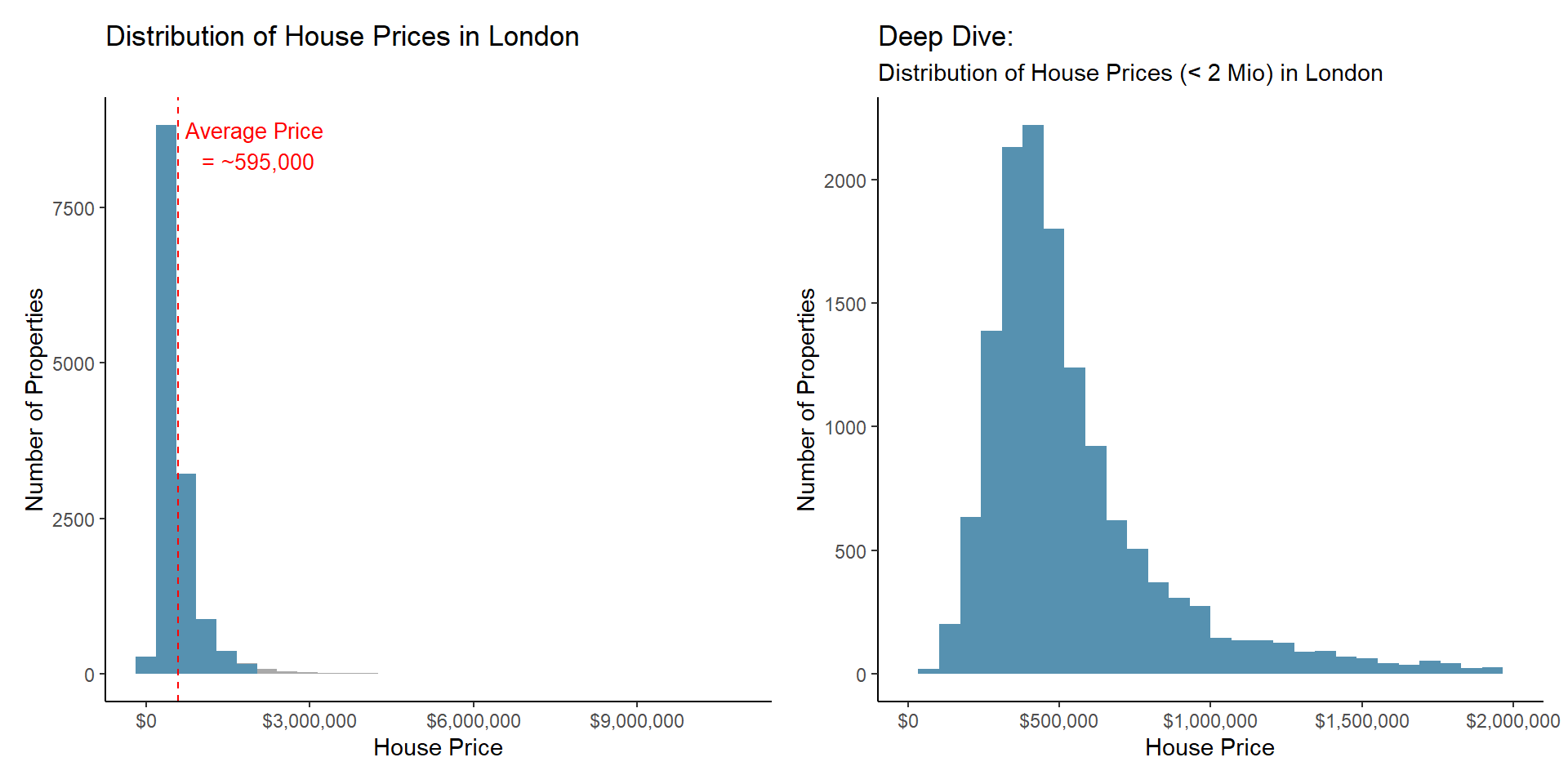
Second, I plot the average price per property type as well as the frequency of each property type. While detached houses, the least frequent sold property type, are on average more expensive, Flats, the most frequent sold property type, are on average the cheapest properties to buy.
p1 <- london_house_prices_2019_training %>%
  group_by(property_type) %>%
  summarise(average_price=mean(price)) %>%
  ggplot(aes(y=average_price, x=reorder(property_type, -average_price), fill=property_type))+
  geom_col()+
  labs(y="Average Price", x="Property Type", title="Average Price per Property Type")+
  scale_x_discrete(labels = c('Detached','Terraced',  'Semi- Detached',"Flats/Maisonettes"))+
  scale_fill_manual(values=c("#317395","#B5D7E9", "#76B3D3", "#5691B0" ))+
  theme_classic()+ #add theme
  theme(legend.position = "none")+
  scale_y_continuous(labels=scales::dollar_format())+
  NULL

p2<- london_house_prices_2019_training %>%
   group_by(property_type) %>%
  summarise(count=n()) %>%
  ggplot(aes(x=reorder(property_type, -count), y=count, fill=property_type))+
    geom_col()+
  scale_x_discrete(labels = c("Flats/Maisonettes",'Terraced',   'Semi- Detached','Detached'))+
  scale_fill_manual(values=c( "#317395","#B5D7E9", "#76B3D3", "#5691B0"))+
   theme(legend.position = "none")+

 scale_y_continuous(label=comma)+
  labs(y="Number of Property Type", x="Property Type", title="Frequency of Property Types sold in 2019")+


  NULL

p1+p2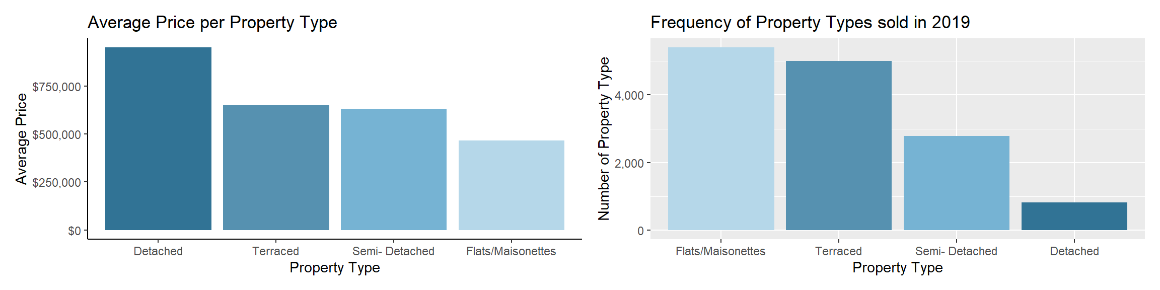
To understand the influence of a property’s size and zone I plot these variables and detect strong relationship between size and price, as well as london zones and prices.
london_house_prices_2019_training %>%
  mutate(london_zone2=as.factor(london_zone)) %>%

  ggplot(aes(y=price, x=total_floor_area, colour=london_zone2))+
 #geom_smooth()+
  geom_point(alpha=0.35)+
  labs(x="Size of Flat (in Sqmtr)", y="Price", title="Positive Relationship between Property' Price and Size", colour="London Zone")+
  theme_classic()+ #add theme
  scale_y_continuous(labels=scales::dollar_format())+

  NULL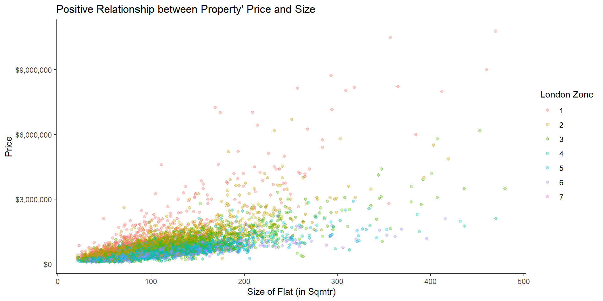
Then, I visualized the positive relationship between average income and price.
london_house_prices_2019_training %>%
  ggplot(aes(y=price, x=average_income))+
  geom_point(alpha=0.35)+
  geom_smooth()+
  labs(x="Average Income", y="Price", title="Relationship between Average Income and Price")+
  theme_classic()+ #add theme
  scale_y_continuous(labels=scales::dollar_format(), limits=c(0, 3000000))+
  scale_x_continuous(label=comma)+
  NULL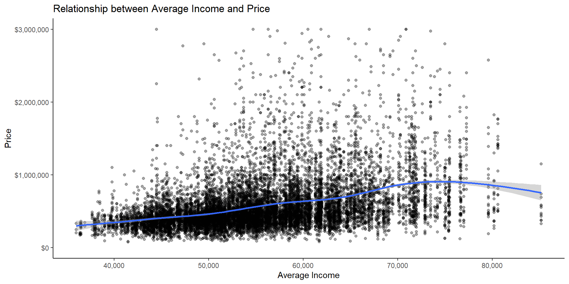
I look at the price/floor area by district.
london_house_prices_2019_training %>%
  mutate(price_floor =price/total_floor_area) %>%
  group_by(district) %>%
  summarise(average_price_floor=mean(price_floor)) %>%
  ggplot(aes(x=average_price_floor, y=reorder(district, average_price_floor)), by_row=TRUE)+
  geom_col()+
  labs(x="Average Price per squaremetre", y="", title="Average Price per District")+
  theme_classic()+ #add theme
  NULL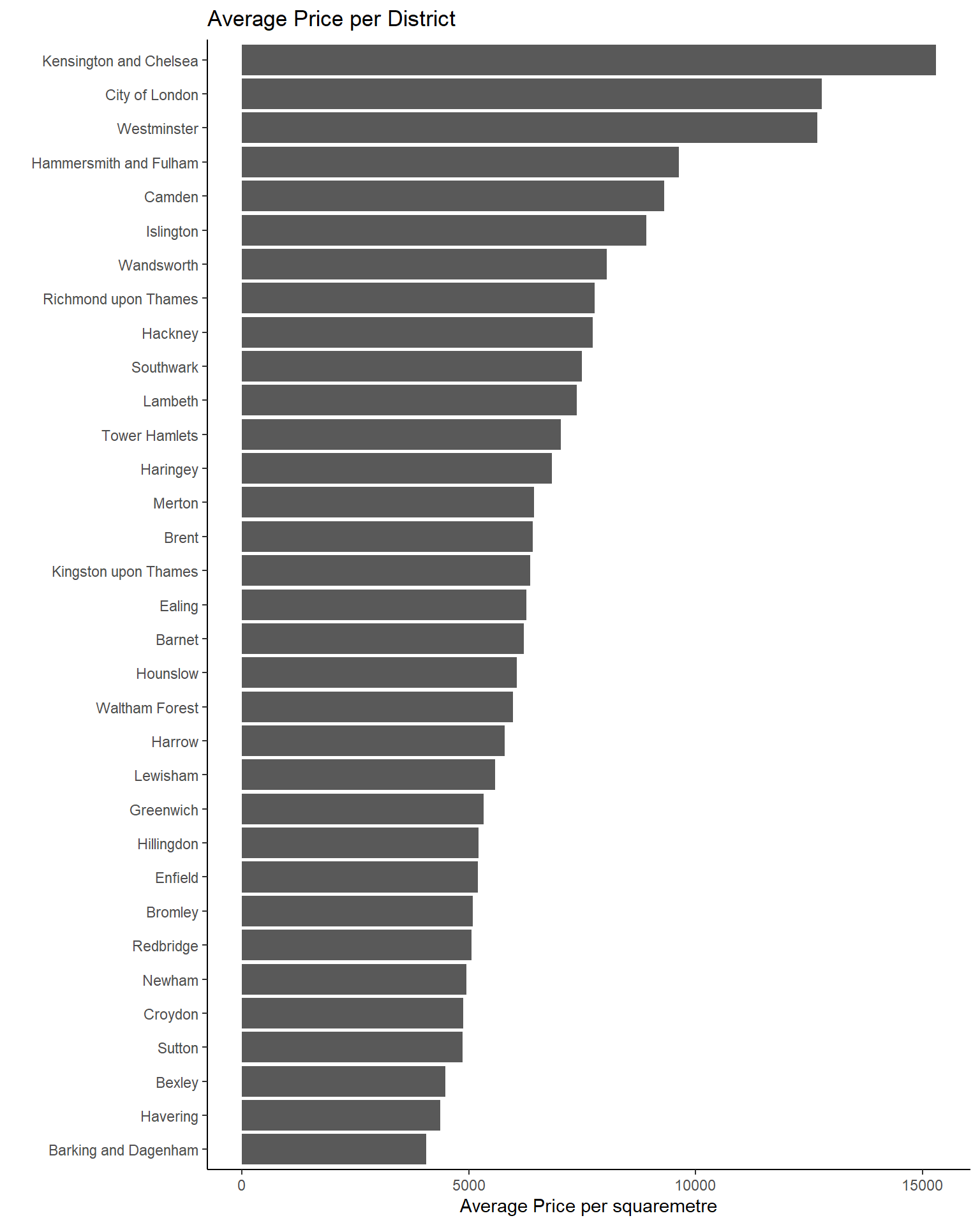
Finally, I check if there are strong correlations between the variables. Some variables such as total floor area, number of habitable rooms, and current CO2 emissions are correlating strongly. Whilst it is important to keep such correlations in mind, they do not constitute a problem when creating models for prediction.
# produce a correlation table using GGally::ggcor()
library("GGally")
london_house_prices_2019_training %>%
select(-ID) %>% #keep Y variable last
ggcorr(method = c("pairwise", "pearson"), layout.exp = 2,label_round=2, label = TRUE,label_size = 2,hjust = 1,nbreaks = 5,size = 2,angle = -20)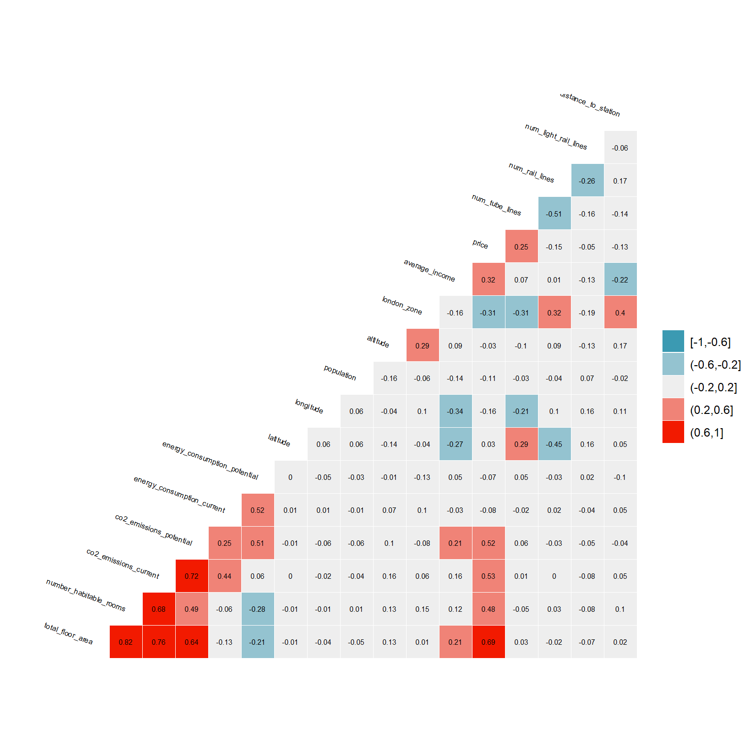 ## Tuning Model
Before creating models, I split the data into training and testing data. I use the training dataset to build my models and test them subsequently on the testing data. Having an outcome variable for the testing data, I can detect if my model overfits before using it for predictions on unlabeled data (houses with no transaction price).
#let's do the initial split
set.seed(1)
library(rsample)
train_test_split <- initial_split(london_house_prices_2019_training, prop = 0.75) #training set contains 75% of the data
train_data <- training(train_test_split)
test_data <- testing(train_test_split)
As first step, I set seed and stabilize a cross-fold validation that I use for all my models. Cross-fold validation is a technique to test the predictive power of a model on a dataset that was not used to create the model, when having a limited number of observations. The seed instead makes it possible to replicate the model with exact the same results.
#Define control variables
set.seed(1)#because I use cross-validation and want to be able to replicate the model
control <- trainControl (
    method="cv", #cross-fold validation
    number=10,
    verboseIter=TRUE) #by setting this to true the model will report its progress after each estimation
I tune all the models maximizing R² and minimizing RMSE. R² is the amount of variance in the data explained by the model. If my model has an R² of 80% for example, the model explains 80% of the different prices between the houses in my dataset. RMSE on the other side, stands for the root mean squared error and is the prediction error of the model.
Linear Regression
The first model I create, is a linear regression. A linear regression looks for the line of best fit between all the variables. I use a stepwise regression when selecting the variables, meaning that I include all of them and subsequently remove unsignificant ones. The only variables I exclude since the beginning are illogical variables such as latitude and longitude, variables with missing data, and variables that are missing in the dataset on which I will do the final predictions. Latitude and longitude are illogical for a linear regression because I assume prices to be higher in the centre if London, and a linear correlation between longitude/latitude and price would therefore be unlikely.
1 Linear Regression
#we are going to train the model and report the results using k-fold cross validation
model_lm_0<-train(
    price ~

   num_tube_lines
   +num_rail_lines
   +num_light_rail_lines
   +distance_to_station
   #+nearest_station #not using it because of new station
   +type_of_closest_station

    +whether_old_or_new
    +freehold_or_leasehold


   +london_zone
   #+postcode_short #too many variables
    #+local_aut #not in out of sample data
    +average_income
  # +nearest_station #problems in out of sample

    +total_floor_area
    +number_habitable_rooms
    +property_type
   +tenure

    +current_energy_rating
   +energy_consumption_potential
   +energy_consumption_current
    +windows_energy_eff
    +co2_emissions_potential
   +co2_emissions_current
    +water_company

    ,
    train_data,
   method = "lm",
    trControl = control
   )

# summary of the results
model_lm_0$result
After excluding all insignificant variables, I create interaction variables between variables that are very important (e.g., total floor area, number of habitable rooms, and London zone), as well as non-linear terms (e.g., (total floor area) ² ) . Then, I replace the geographical categorical variable postcode short with London zones, because while many postcodes turn out to be insignificant, London zones seems to be a good indicator for geographical distribution of prices.
2 Linear Regression
#we are going to train the model and report the results using k-fold cross validation
model_lm<-train(
    price ~
   num_tube_lines

    +district:property_type
    +london_zone*poly(total_floor_area,2)*number_habitable_rooms
    +average_income

    +energy_consumption_potential
   +energy_consumption_current
   +current_energy_rating
    +windows_energy_eff
    +co2_emissions_potential
   +co2_emissions_current
    +water_company
    ,
    train_data,
   method = "lm",
    trControl = control
   )
## + Fold01: intercept=TRUE
## - Fold01: intercept=TRUE
## + Fold02: intercept=TRUE
## - Fold02: intercept=TRUE
## + Fold03: intercept=TRUE
## - Fold03: intercept=TRUE
## + Fold04: intercept=TRUE
## - Fold04: intercept=TRUE
## + Fold05: intercept=TRUE
## - Fold05: intercept=TRUE
## + Fold06: intercept=TRUE
## - Fold06: intercept=TRUE
## + Fold07: intercept=TRUE
## - Fold07: intercept=TRUE
## + Fold08: intercept=TRUE
## - Fold08: intercept=TRUE
## + Fold09: intercept=TRUE
## - Fold09: intercept=TRUE
## + Fold10: intercept=TRUE
## - Fold10: intercept=TRUE
## Aggregating results
## Fitting final model on full training set# summary of the results
model_lm$result## intercept RMSE Rsquared MAE RMSESD RsquaredSD MAESD
## 1 TRUE 233128 0.804 117778 40439 0.0284 7436Then, I plot the results of the final model as well as the importance of each variable:
model_lm$results## intercept RMSE Rsquared MAE RMSESD RsquaredSD MAESD
## 1 TRUE 233128 0.804 117778 40439 0.0284 7436# we can check variable importance as well
importance <- varImp(model_lm, scale=TRUE)
plot(importance)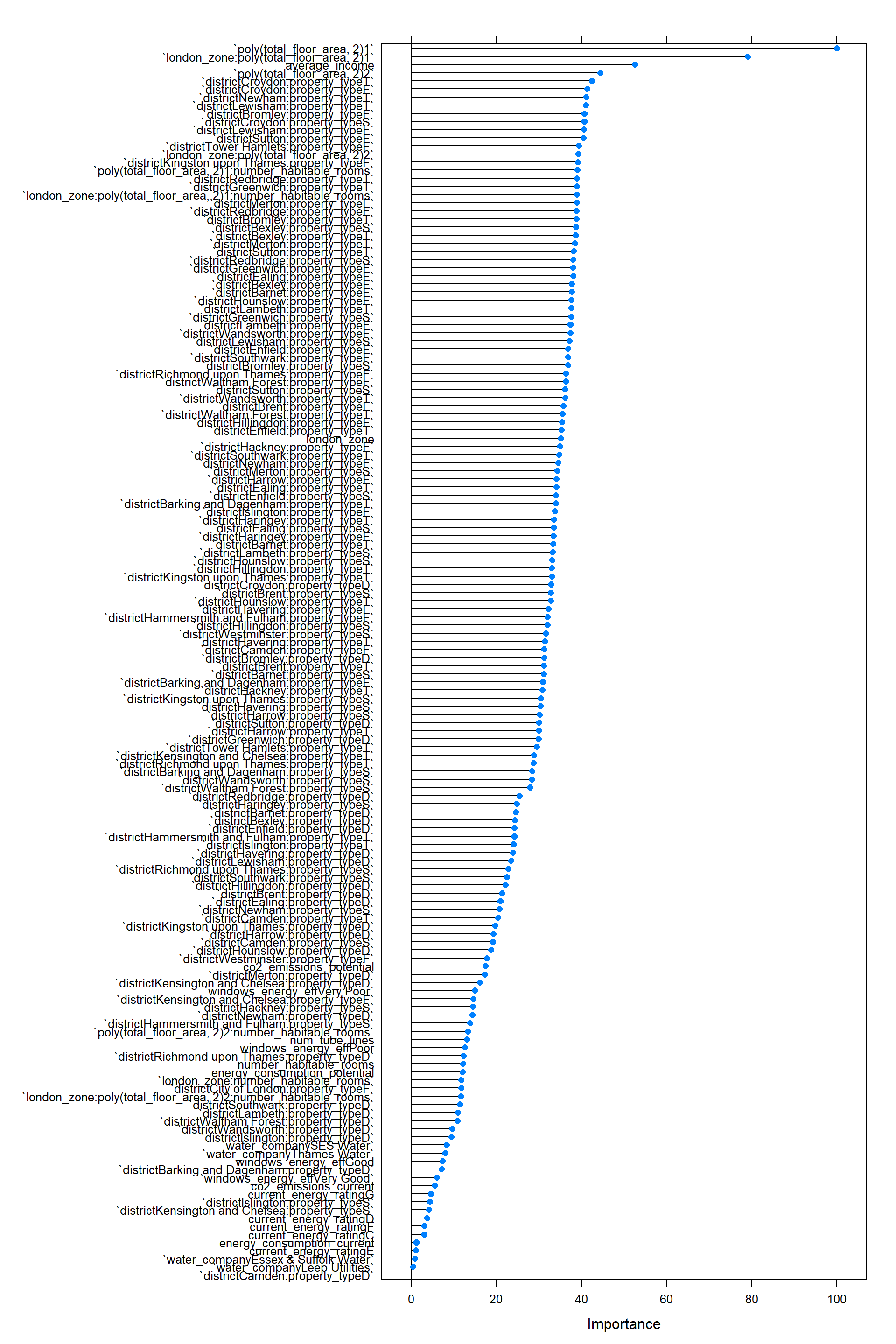
Prediction lm
Below I use the predict function to test the performance of the model in testing data and summarize the performance of the linear regression model.
# We can predict the testing values

predictions_lm <- predict(model_lm,test_data)

lm_results<-data.frame(RMSE = RMSE(predictions_lm, test_data$price), #how much did qe predict wrong
                            Rsquare = R2(predictions_lm, test_data$price)) #how much does the model cover
lm_results
## RMSE Rsquare
## 1 208392 0.835The performance of the model (in R²): - Training 0.8102 - Testing 0.8358638
LASSO
As second model, I performed a LASSO regression using the same variables as in the linear regression. LASSO regression is a type of linear regression that shirks the impact of the variables (regularization) and eliminates insignificant variables (parameter selection). To do so, I introduce artificially a bias (lambda) which adds a penalty to the coefficients for each variable. As consequence, all variables have a lower coefficient, and some go down to zero, resulting into a simpler model with less variance but a higher bias. I optimize the model calculating the error of the model (RMSE – root mean standard error) as well as the explanatory power of my model (R²) for different biases (lambda). Finally, I select the model with the lowest RMSE and highest R².
#split data into training & testing -> already done
#we need to optimize the lambda in this sequence
lambda_seq <- seq(0, 1000, length =100)

#we use cross fold validation
set.seed(1)
control <- trainControl(
  method="cv",
  number = 10,
  verboseIter = FALSE)

#LASSO regression to select the best lambda
set.seed(1)
lasso_fit <- train(price ~
    #  distance_to_station #not significant
    num_tube_lines #not significant

    +whether_old_or_new #not significant
    +freehold_or_leasehold #not significant

    +distance_to_station
    +district:property_type
    +london_zone*poly(total_floor_area,2)*number_habitable_rooms

    +average_income

    +energy_consumption_potential
    +energy_consumption_current #new
    +current_energy_rating #new
    +windows_energy_eff
    +co2_emissions_potential
    +co2_emissions_current #new
    +water_company,

        data=train_data,
        method="glmnet",
        preProc = c("center", "scale"), #This option standardizes the data before running the LASSO regression if alpha = 0 ->RIDGE REG

   trControl = control,
  tuneGrid = expand.grid(alpha = 1, lambda = lambda_seq) #alpha=1 specifies to run a LASSO regression. If alpha=0 the model would run ridge regression.

)

coef(lasso_fit$finalModel, lasso_fit$bestTune$lambda)
## 166 x 1 sparse Matrix of class "dgCMatrix"
## 1
## (Intercept) 594480.4
## num_tube_lines 15627.7
## whether_old_or_newY 224.5
## freehold_or_leaseholdL -16424.4
## distance_to_station -2672.4
## london_zone -183472.0
## poly(total_floor_area, 2)1 1014162.8
## poly(total_floor_area, 2)2 321756.7
## number_habitable_rooms -77333.0
## average_income 60282.3
## energy_consumption_potential -31968.4
## energy_consumption_current -3455.7
## current_energy_ratingC 7340.9
## current_energy_ratingD 11157.3
## current_energy_ratingE 1872.5
## current_energy_ratingF -6706.5
## current_energy_ratingG -6338.3
## windows_energy_effGood 6860.1
## windows_energy_effPoor 12230.9
## windows_energy_effVery Good 5449.2
## windows_energy_effVery Poor 15294.0
## co2_emissions_potential 52468.6
## co2_emissions_current 19618.9
## water_companyEssex & Suffolk Water 1951.1
## water_companyLeep Utilities 480.6
## water_companySES Water 16647.1
## water_companyThames Water 19487.2
## districtBarking and Dagenham:property_typeD 741.2
## districtBarnet:property_typeD 8899.5
## districtBexley:property_typeD 6705.5
## districtBrent:property_typeD 17.9
## districtBromley:property_typeD 4916.5
## districtCamden:property_typeD 20854.7
## districtCity of London:property_typeD .
## districtCroydon:property_typeD .
## districtEaling:property_typeD -2317.4
## districtEnfield:property_typeD 1697.5
## districtGreenwich:property_typeD -2060.0
## districtHackney:property_typeD .
## districtHammersmith and Fulham:property_typeD .
## districtHaringey:property_typeD .
## districtHarrow:property_typeD 15067.9
## districtHavering:property_typeD 8804.1
## districtHillingdon:property_typeD 11477.0
## districtHounslow:property_typeD -1948.6
## districtIslington:property_typeD 3586.6
## districtKensington and Chelsea:property_typeD 26187.9
## districtKingston upon Thames:property_typeD 17165.4
## districtLambeth:property_typeD .
## districtLewisham:property_typeD -3538.1
## districtMerton:property_typeD 7032.9
## districtNewham:property_typeD -830.4
## districtRedbridge:property_typeD -505.6
## districtRichmond upon Thames:property_typeD 21716.2
## districtSouthwark:property_typeD 1695.9
## districtSutton:property_typeD -2205.3
## districtTower Hamlets:property_typeD .
## districtWaltham Forest:property_typeD -2466.1
## districtWandsworth:property_typeD 1418.8
## districtWestminster:property_typeD .
## districtBarking and Dagenham:property_typeF -2026.1
## districtBarnet:property_typeF -3295.1
## districtBexley:property_typeF -6900.2
## districtBrent:property_typeF 1751.8
## districtBromley:property_typeF -10417.3
## districtCamden:property_typeF 17719.7
## districtCity of London:property_typeF 6747.4
## districtCroydon:property_typeF -11591.3
## districtEaling:property_typeF -3341.8
## districtEnfield:property_typeF -3003.8
## districtGreenwich:property_typeF -4605.3
## districtHackney:property_typeF 5717.0
## districtHammersmith and Fulham:property_typeF 6835.5
## districtHaringey:property_typeF 2921.2
## districtHarrow:property_typeF -3248.2
## districtHavering:property_typeF -1685.6
## districtHillingdon:property_typeF -2903.0
## districtHounslow:property_typeF -4087.1
## districtIslington:property_typeF 7575.7
## districtKensington and Chelsea:property_typeF 58576.9
## districtKingston upon Thames:property_typeF -6698.3
## districtLambeth:property_typeF 190.1
## districtLewisham:property_typeF -9213.2
## districtMerton:property_typeF -5475.4
## districtNewham:property_typeF -2019.2
## districtRedbridge:property_typeF -6521.9
## districtRichmond upon Thames:property_typeF -1321.1
## districtSouthwark:property_typeF 3226.7
## districtSutton:property_typeF -13613.8
## districtTower Hamlets:property_typeF -5952.0
## districtWaltham Forest:property_typeF -377.0
## districtWandsworth:property_typeF 432.1
## districtWestminster:property_typeF 51586.5
## districtBarking and Dagenham:property_typeS -2821.9
## districtBarnet:property_typeS 9386.9
## districtBexley:property_typeS -9391.0
## districtBrent:property_typeS 941.9
## districtBromley:property_typeS -4364.0
## districtCamden:property_typeS 4957.4
## districtCity of London:property_typeS .
## districtCroydon:property_typeS -14299.3
## districtEaling:property_typeS 545.1
## districtEnfield:property_typeS 229.0
## districtGreenwich:property_typeS -8143.4
## districtHackney:property_typeS 4730.4
## districtHammersmith and Fulham:property_typeS 4410.2
## districtHaringey:property_typeS -583.5
## districtHarrow:property_typeS 3694.2
## districtHavering:property_typeS 6868.8
## districtHillingdon:property_typeS 5663.6
## districtHounslow:property_typeS 732.9
## districtIslington:property_typeS 10416.9
## districtKensington and Chelsea:property_typeS 21702.0
## districtKingston upon Thames:property_typeS 6164.4
## districtLambeth:property_typeS -5793.6
## districtLewisham:property_typeS -9075.0
## districtMerton:property_typeS -3421.5
## districtNewham:property_typeS -1764.4
## districtRedbridge:property_typeS -8344.5
## districtRichmond upon Thames:property_typeS 18367.4
## districtSouthwark:property_typeS 4246.4
## districtSutton:property_typeS -7473.4
## districtTower Hamlets:property_typeS .
## districtWaltham Forest:property_typeS 2508.4
## districtWandsworth:property_typeS .
## districtWestminster:property_typeS 36645.3
## districtBarking and Dagenham:property_typeT -3750.0
## districtBarnet:property_typeT 2038.4
## districtBexley:property_typeT -9459.4
## districtBrent:property_typeT 5873.7
## districtBromley:property_typeT -9290.5
## districtCamden:property_typeT 17439.6
## districtCity of London:property_typeT .
## districtCroydon:property_typeT -19230.9
## districtEaling:property_typeT 925.4
## districtEnfield:property_typeT -909.1
## districtGreenwich:property_typeT -8340.4
## districtHackney:property_typeT 5746.9
## districtHammersmith and Fulham:property_typeT 19177.7
## districtHaringey:property_typeT 3045.0
## districtHarrow:property_typeT 945.0
## districtHavering:property_typeT 3049.0
## districtHillingdon:property_typeT -95.0
## districtHounslow:property_typeT 3878.1
## districtIslington:property_typeT 11445.4
## districtKensington and Chelsea:property_typeT 104020.5
## districtKingston upon Thames:property_typeT 1782.9
## districtLambeth:property_typeT -6490.8
## districtLewisham:property_typeT -13920.0
## districtMerton:property_typeT -7423.7
## districtNewham:property_typeT -13263.4
## districtRedbridge:property_typeT -9798.2
## districtRichmond upon Thames:property_typeT 15582.9
## districtSouthwark:property_typeT .
## districtSutton:property_typeT -11001.5
## districtTower Hamlets:property_typeT -551.7
## districtWaltham Forest:property_typeT 398.7
## districtWandsworth:property_typeT 456.0
## districtWestminster:property_typeT 35411.7
## london_zone:poly(total_floor_area, 2)1 -791217.7
## london_zone:poly(total_floor_area, 2)2 -272639.0
## london_zone:number_habitable_rooms 103682.4
## poly(total_floor_area, 2)1:number_habitable_rooms -401559.0
## poly(total_floor_area, 2)2:number_habitable_rooms -68996.2
## london_zone:poly(total_floor_area, 2)1:number_habitable_rooms 399638.7
## london_zone:poly(total_floor_area, 2)2:number_habitable_rooms 57036.3Predict lasso
#lasso_fit$results
plot(lasso_fit)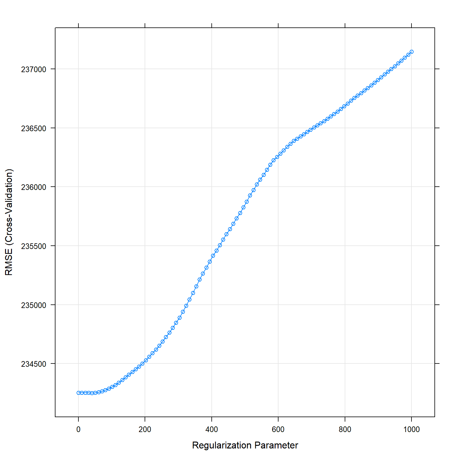
predictions_lasso <- predict(lasso_fit, test_data)
lasso_results <- data.frame( RMSE =RMSE(predictions_lasso, test_data$price),
                             Rsquare =R2(predictions_lasso, test_data$price))

lasso_results
## RMSE Rsquare
## 1 207501 0.836The performance of the model (in R²): - Training: 0.8026139 - Testing: 0.8360793
KNN
As third model I use the k-Nearest Neighbours (k-NN) model. It predicts a value based on a datapoint’s k nearest neighbours. This means, that the price of a property is predicted based on the k most similar properties in the training dataset. To select the variables, I use the knowledge gained from the linear regression and take the significant variables from the linear regression. Furthermore, I include latitude and longitude as this model does not assume a linear relationship between the dependent and the independent variable. Finally, I remove the interaction variables given this model’s ability in determining them by itself. Before running the model, I make sure to standardize the variables, as the distance between the points should not be influenced by different units of the variables. Then, I optimize my model using different numbers for the number of neighbours (k).
To do so, I first use 10 random values for k with tuneLength, and then optimize for values close to the best performing k-value with tuneGrid.
KNN: 10 random values for k
#knn
# selecting the best k with the highest R²
set.seed(1) #because I use cross-validation and want to be able to replicate the model

knn_fit_1 <- train(
  price ~

        #  distance_to_station #not significant
   num_tube_lines #not significant

    +latitude
    +longitude

    +district
    +property_type
    +london_zone
    +total_floor_area
    +number_habitable_rooms
    +average_income

    +energy_consumption_potential
    +windows_energy_eff
    +co2_emissions_potential
    +water_company
  ,
  train_data,

                method = "knn",
                 trControl = control, #use the same as I used in linear regression
                 tuneLength = 10, #number of parameter values train function will try
                 preProcess = c("center", "scale"), #center and scale the data in k-nn this is pretty important
                 metric="RMSE" #default metric is accuracy, I change it to R²

  )

print(knn_fit_1)
## k-Nearest Neighbors
##
## 10499 samples
## 13 predictor
##
## Pre-processing: centered (52), scaled (52)
## Resampling: Cross-Validated (10 fold)
## Summary of sample sizes: 9450, 9450, 9449, 9448, 9450, 9449, ...
## Resampling results across tuning parameters:
##
## k RMSE Rsquared MAE
## 5 267358 0.746 125679
## 7 268003 0.750 124951
## 9 268917 0.754 125417
## 11 272270 0.753 126574
## 13 275337 0.750 127294
## 15 278772 0.746 128228
## 17 279448 0.749 128974
## 19 280789 0.749 129780
## 21 283118 0.748 130544
## 23 285960 0.745 131288
##
## RMSE was used to select the optimal model using the smallest value.
## The final value used for the model was k = 5.plot(knn_fit_1)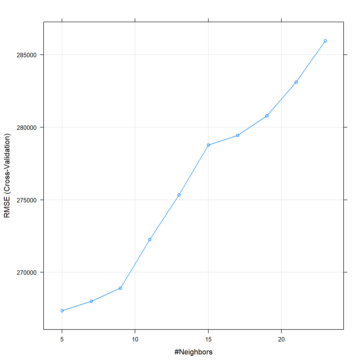
KNN: tuneGrid
The best k seems to be between 1 and 7, therefore I use tuneGrid to get the best k.
#knn2
Grid_knn <- expand.grid(k=seq(1, 7, 1))
# selecting the best k with the highest R²
set.seed(1) #because I use cross-validation and want to be able to replicate the model

knn_fit_2 <- train(
  price ~

        #  distance_to_station #not significant
   num_tube_lines #not significant

    +latitude
    +longitude

    +district
    +property_type
    +london_zone
    +total_floor_area
    +number_habitable_rooms
    +average_income

    +energy_consumption_potential
    +windows_energy_eff
    +co2_emissions_potential
    +water_company
  ,
  train_data,

    method = "knn",
     trControl = control, #use the same as I used in linear regression
     tuneGrid = Grid_knn, #looking for numbers around
     preProcess = c("center", "scale"), #center and scale the data in k-nn this is pretty important
     metric="RMSE") #default metric is accuracy is binary, otherwise RMSE, I change it to R²

print(knn_fit_2)
## k-Nearest Neighbors
##
## 10499 samples
## 13 predictor
##
## Pre-processing: centered (52), scaled (52)
## Resampling: Cross-Validated (10 fold)
## Summary of sample sizes: 9450, 9450, 9449, 9448, 9450, 9449, ...
## Resampling results across tuning parameters:
##
## k RMSE Rsquared MAE
## 1 313051 0.658 149998
## 2 281924 0.709 134824
## 3 275575 0.725 130291
## 4 271762 0.734 127669
## 5 267358 0.746 125679
## 6 265788 0.752 124721
## 7 268003 0.750 124951
##
## RMSE was used to select the optimal model using the smallest value.
## The final value used for the model was k = 6.plot(knn_fit_2)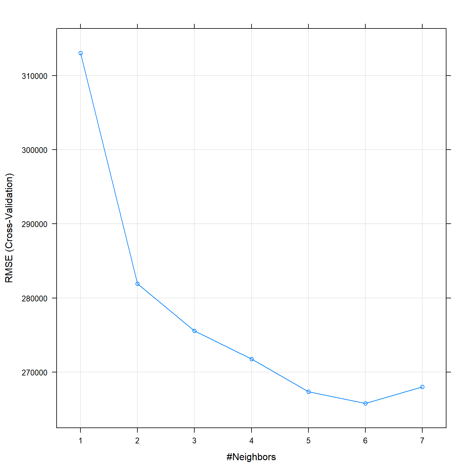
Prediction KNN
#predict the price of each house in the test data set
#recall that the output of "train" function (knn_fit) automatically keeps the best model
knn_prediction <- predict(knn_fit_2, newdata = test_data)

knn_results<-data.frame(RMSE = RMSE(knn_prediction, test_data$price), Rsquare = R2(knn_prediction, test_data$price))

knn_results
## RMSE Rsquare
## 1 260115 0.751The number of neighbors that optimize RMSE are k=6.
The performance of the model (in R²): - training:0.7524809 - testing: 0.7509709
Regression Tree Model
The fourth model is a regression tree and splits the data base multiple times based on various variables with respective cut-off values. After each split, subsets are created that are again divided based on another variable. The splitting stops after a predefined number of splits or other parameters that can be pre-set. One of these parameters, is the complexity parameter (cp) that stabilizes that a split is executed, only if the cost this additional split is below its value. I optimized the model (low RMSE and high R²) for this parameter. This model detects relationships between variables as well as nonlinear variables. Consequently, I do not need to create interaction variables myself. I use all the significant variables from the linear regression but remove the interactions between them. On the other side, this model is not as good in detecting linear relationships and is a very unstable method due to overfitting (high variance). This means if the data changes even slightly they can fit very different models.
Tree 1
#no need to scale the data

set.seed(12) #because I use cross-validation and want to be able to replicate the model
model_tree_1 <- train(
  price ~

        #  distance_to_station #not significant
   num_tube_lines #not significant

    +latitude
    +longitude

    +district
    +property_type
    +london_zone
    +total_floor_area
    +number_habitable_rooms
    +average_income

    +energy_consumption_potential
    +windows_energy_eff
    +co2_emissions_potential
    +water_company
  ,
  train_data,
  method = "rpart",
  metric= "RMSE",
  trControl = control, #I use the same as in lm
  tuneLength= 30

    )

#You can view how the tree performs
model_tree_1$results
## cp RMSE Rsquared MAE RMSESD RsquaredSD MAESD
## 1 0.00164 264365 0.742 141511 38949 0.0554 5740
## 2 0.00186 266556 0.738 142519 39248 0.0550 5941
## 3 0.00198 267970 0.735 143592 39405 0.0556 6322
## 4 0.00202 268254 0.735 143988 39548 0.0559 6702
## 5 0.00273 272978 0.726 147145 38766 0.0526 7032
## 6 0.00283 273553 0.725 147789 39076 0.0525 7533
## 7 0.00289 273818 0.725 148295 38975 0.0521 7398
## 8 0.00318 276656 0.719 150837 39662 0.0559 7903
## 9 0.00408 278710 0.714 152584 38184 0.0530 7414
## 10 0.00443 281791 0.708 153687 39279 0.0513 7013
## 11 0.00456 282010 0.708 153932 39086 0.0518 6708
## 12 0.00462 282636 0.707 154158 39313 0.0526 6738
## 13 0.00510 285748 0.701 155335 40228 0.0553 6965
## 14 0.00571 288520 0.695 156575 41560 0.0596 7778
## 15 0.00619 293865 0.682 157678 41021 0.0672 7851
## 16 0.00632 294350 0.680 158019 40738 0.0679 7639
## 17 0.00798 297009 0.675 162522 42001 0.0736 7525
## 18 0.00857 299525 0.670 164962 44730 0.0729 8582
## 19 0.00891 300604 0.667 165095 44285 0.0747 8356
## 20 0.00966 303419 0.659 168440 44942 0.0764 9998
## 21 0.01282 315338 0.632 174684 44254 0.0797 11046
## 22 0.01352 319583 0.621 177083 42237 0.0855 10596
## 23 0.01359 319583 0.621 177083 42237 0.0855 10596
## 24 0.01832 327989 0.601 183778 41518 0.0846 8308
## 25 0.02398 332593 0.589 185846 41072 0.0773 8996
## 26 0.03224 345498 0.563 188729 45582 0.0573 9130
## 27 0.04310 358185 0.527 196768 42264 0.0782 9802
## 28 0.07590 376073 0.474 215196 36290 0.0903 13055
## 29 0.16197 422396 0.345 235651 66448 0.0874 13000
## 30 0.31416 465807 0.276 254039 70395 0.0327 26705#summary(model2_tree)
#You can view the final tree
rpart.plot(model_tree_1$finalModel)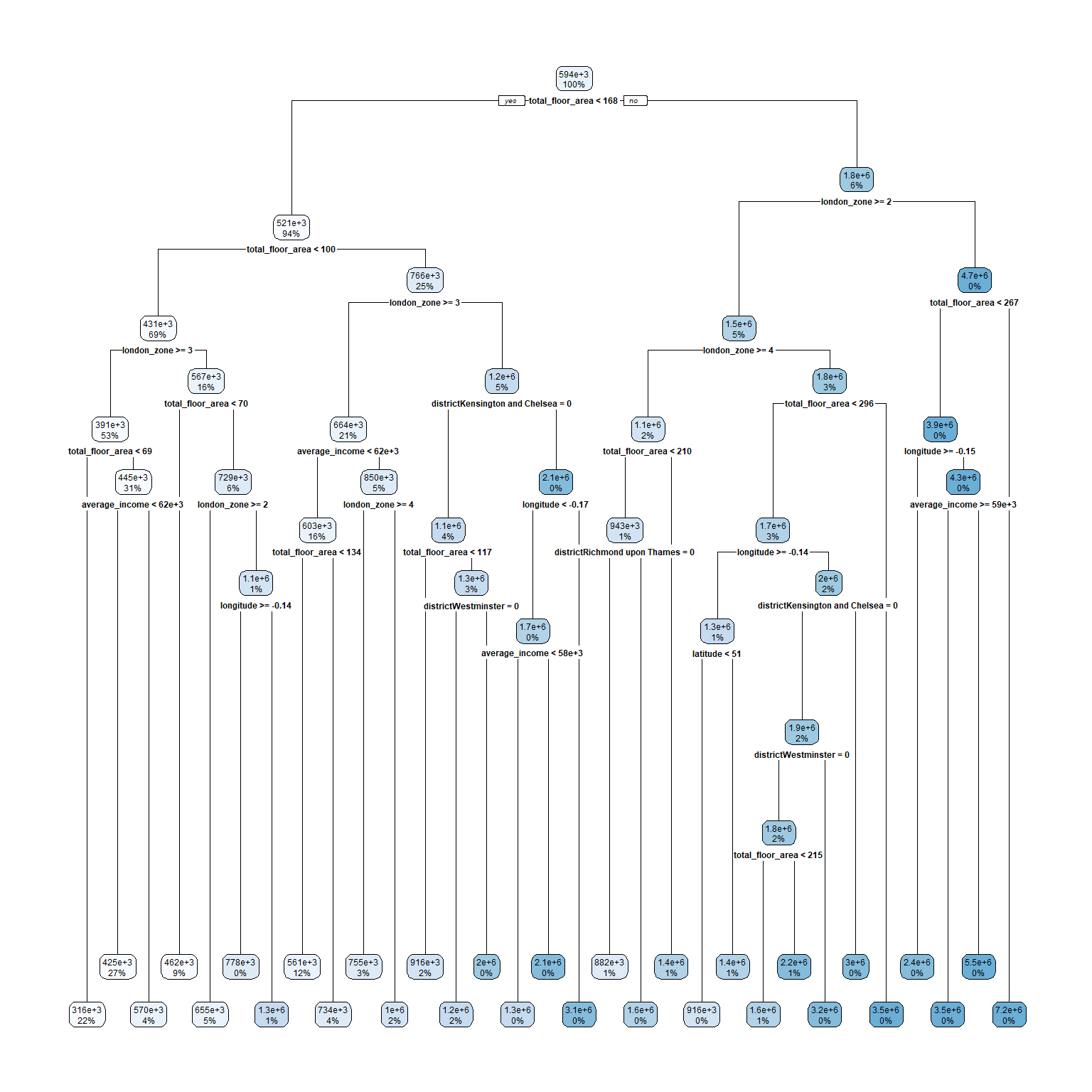
#you can also visualize the variable importance
importance <- varImp(model_tree_1, scale=TRUE)
plot(importance)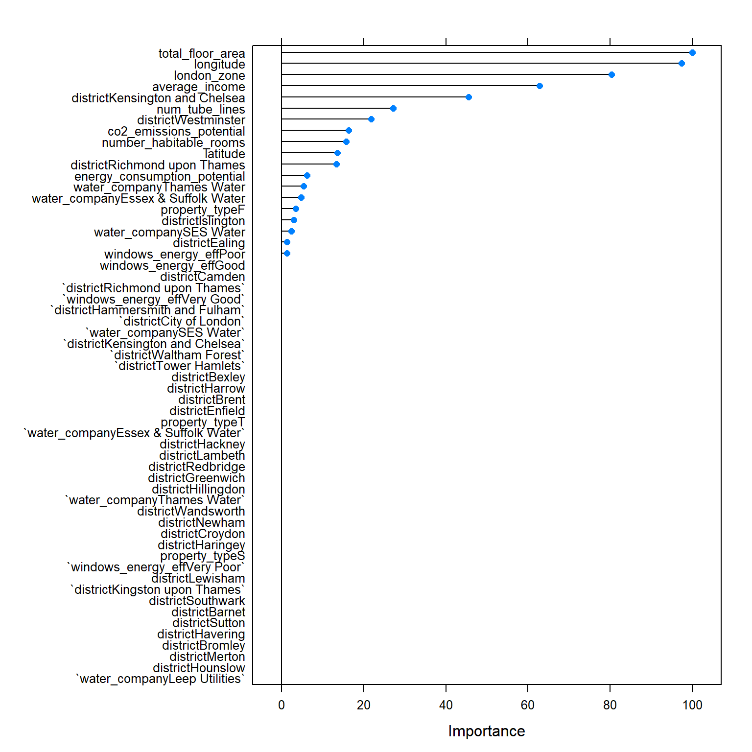
Tree 2
The best cp seems to be between 0.000 and 0.0001, therefore I use tuneGrid to get the best cp.
#no need to scale the data

#run model
set.seed(1) #because I use cross-validation and want to be able to replicate the model
model_tree_2 <- train(
  price ~

        #  distance_to_station #not significant
   num_tube_lines #not significant

    +latitude
    +longitude

    +district
    +property_type
    +london_zone
    +total_floor_area
    +number_habitable_rooms
    +average_income

    +energy_consumption_potential
    +windows_energy_eff
    +co2_emissions_potential
    +water_company
  ,
  train_data,


  method = "rpart",
  metric="RMSE",
  trControl = control, #I use the same as in lm
  tuneGrid= expand.grid(cp=seq(0.000, 0.0001, 0.00001))
    )

#You can view how the tree performs
model_tree_2$results
## cp RMSE Rsquared MAE RMSESD RsquaredSD MAESD
## 1 0e+00 243218 0.786 117368 38730 0.0502 6176
## 2 1e-05 242872 0.787 116591 38809 0.0500 6334
## 3 2e-05 242700 0.787 116504 38766 0.0497 6220
## 4 3e-05 242835 0.787 116555 38590 0.0498 6031
## 5 4e-05 243097 0.786 117376 38655 0.0500 6023
## 6 5e-05 243311 0.785 117656 38492 0.0499 5799
## 7 6e-05 243437 0.785 117937 38576 0.0500 6003
## 8 7e-05 243507 0.785 118145 38853 0.0507 6221
## 9 8e-05 243700 0.784 118314 38962 0.0517 6125
## 10 9e-05 243853 0.784 118551 38927 0.0523 6049
## 11 1e-04 243958 0.784 118951 38977 0.0526 6112#summary(model_tree_2)
plot(model_tree_2)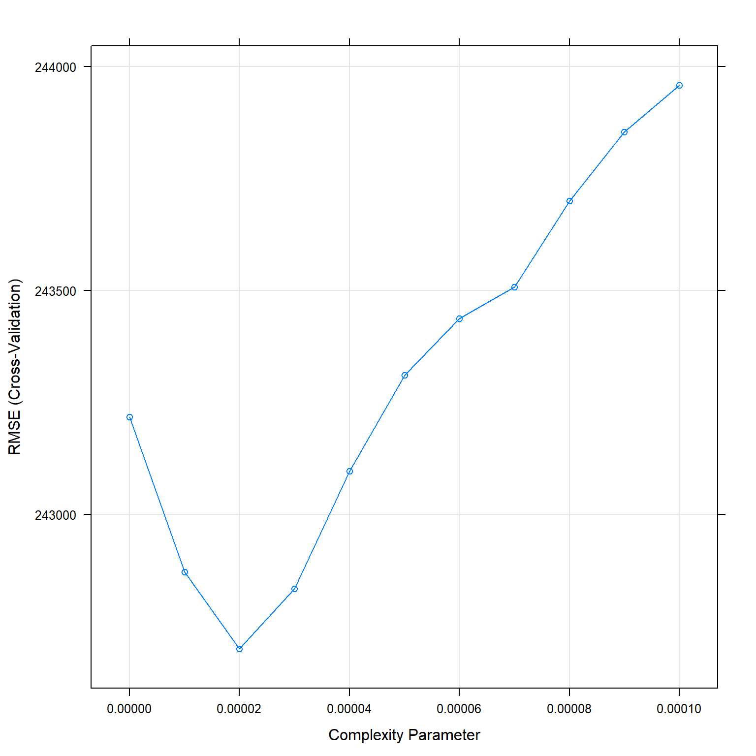
#You can view the final tree
rpart.plot(model_tree_2$finalModel)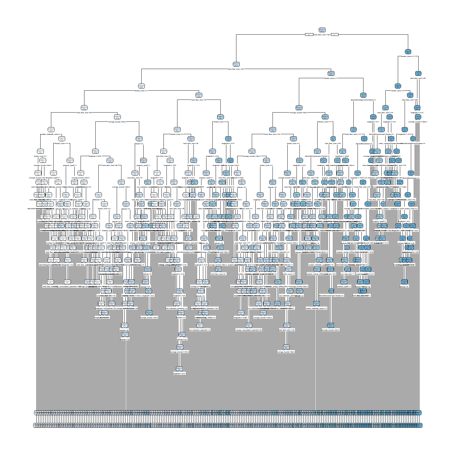
#you can also visualize the variable importance
importance <- varImp(model_tree_2, scale=TRUE)
plot(importance)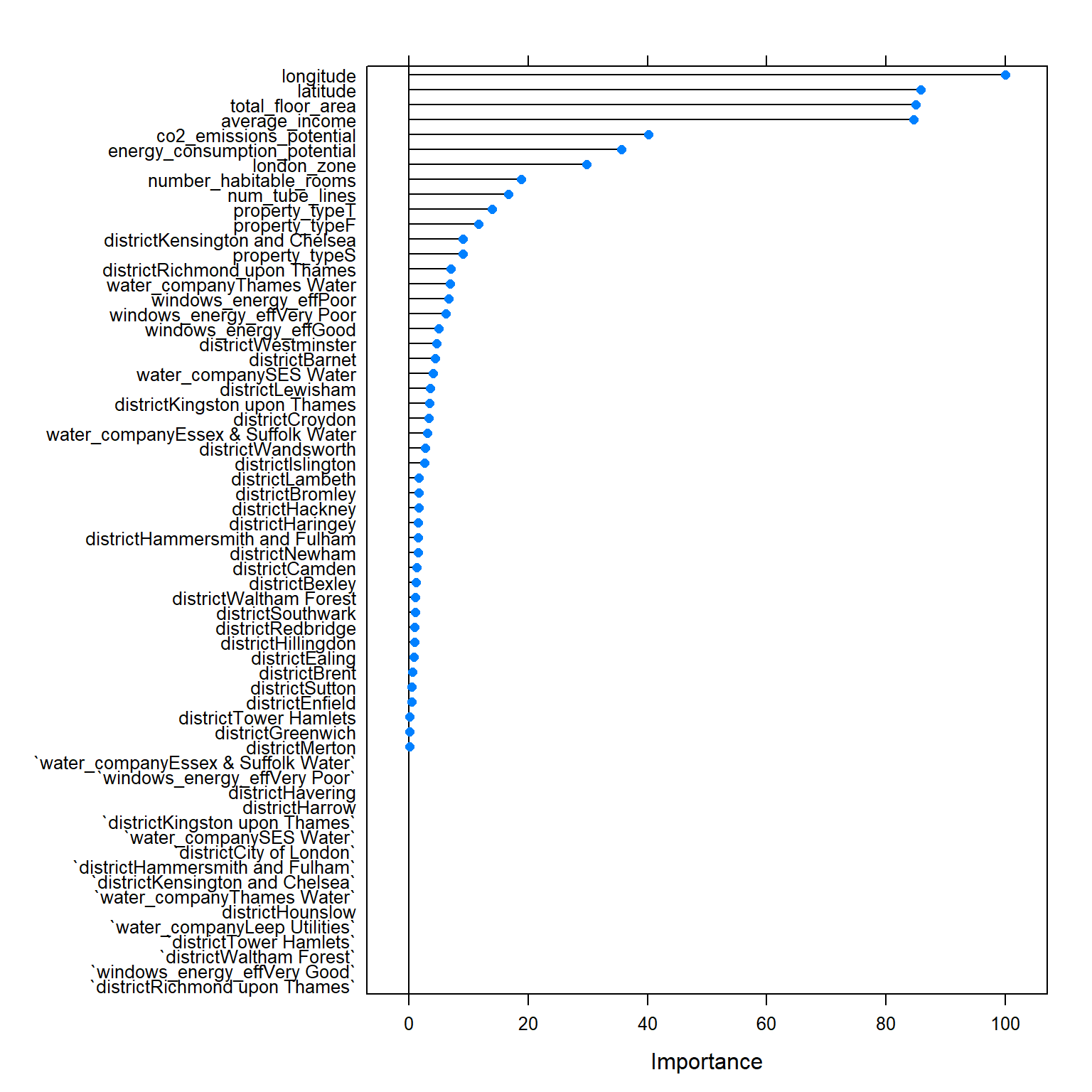
RSquared is 0.7869522 for cp = 0.00002
Prediction
# We can predict the testing values
predictions_tree <- predict(model_tree_2,test_data)

tree_results<-data.frame(RMSE = RMSE(predictions_tree, test_data$price), #how much did qe predict wrong
                            Rsquare = R2(predictions_tree, test_data$price)) #how much does the model cover
tree_results
## RMSE Rsquare
## 1 229721 0.8The performance of the model (in R²): - Training R² 0.7869522 - Testing R² is 0.8000181.
We need to be careful about making conclusions based on model trees because there is a high variance. This means if the data changes even slightly they can fit very different models. (you could test this using different seeds)
Random Forest
Random Forest is an ensembled learning method that creates multiple trees and takes the average of the individual trees’ predictions as prediction. It corrects the tendency of regression trees to overfitt to their training dataset. To optimize RMSE and R² for the random trees, I tuned the number of variables to possibly split at in each node and as split rule I selected “variance” as opposed to “extratrees”. To save computational power I used 5 as a minimum node size (which is the default option for prediction).
RF 1
#random forest is an assembled method

set.seed(1)
rf_fit <- train(
  price ~

        #  distance_to_station #not significant
   num_tube_lines #not significant

    +latitude
    +longitude

    +district
    +property_type
    +london_zone
    +total_floor_area
    +number_habitable_rooms
    +average_income

    +energy_consumption_potential
    +windows_energy_eff
    +co2_emissions_potential
    +water_company
  ,
  train_data,


  method = "ranger",
  metric="RMSE",
  trControl = control,
  tuneLength= 10,
  importance = 'permutation')

print(rf_fit)
## Random Forest
##
## 10499 samples
## 13 predictor
##
## No pre-processing
## Resampling: Cross-Validated (10 fold)
## Summary of sample sizes: 9450, 9450, 9449, 9448, 9450, 9449, ...
## Resampling results across tuning parameters:
##
## mtry splitrule RMSE Rsquared MAE
## 2 variance 326210 0.768 155557
## 2 extratrees 367703 0.710 180575
## 7 variance 219461 0.840 98794
## 7 extratrees 239633 0.815 106881
## 13 variance 206101 0.850 95272
## 13 extratrees 216523 0.838 97900
## 18 variance 203677 0.852 95053
## 18 extratrees 210693 0.844 96271
## 24 variance 202533 0.852 95173
## 24 extratrees 208625 0.845 95546
## 29 variance 202227 0.851 95203
## 29 extratrees 207037 0.847 95353
## 35 variance 201855 0.851 95260
## 35 extratrees 205923 0.848 95334
## 40 variance 202009 0.851 95441
## 40 extratrees 207782 0.844 95555
## 46 variance 202827 0.849 95701
## 46 extratrees 205341 0.848 95319
## 52 variance 202402 0.850 95710
## 52 extratrees 205920 0.846 95628
##
## Tuning parameter 'min.node.size' was held constant at a value of 5
## RMSE was used to select the optimal model using the smallest value.
## The final values used for the model were mtry = 35, splitrule = variance
## and min.node.size = 5.plot(rf_fit)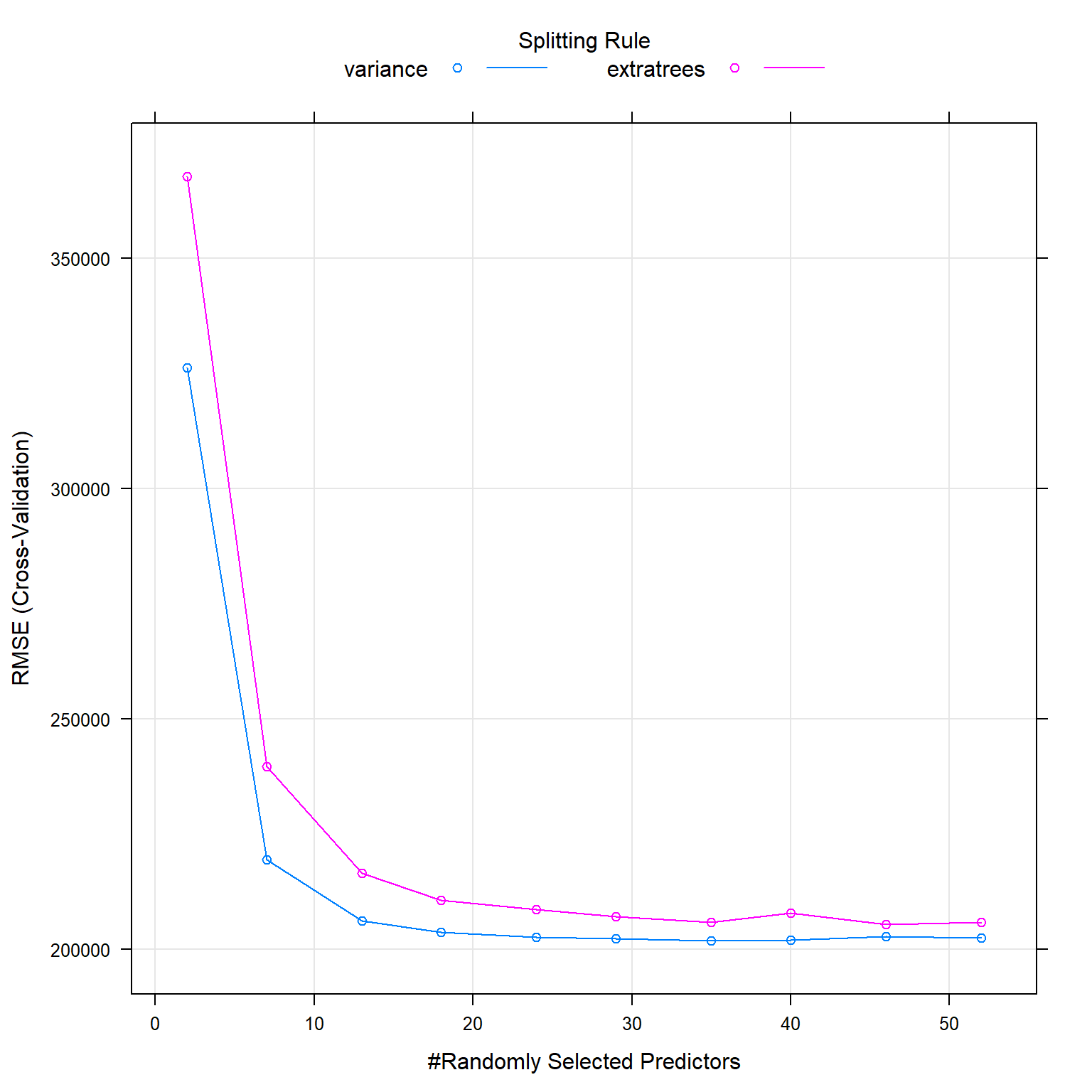
After selecting
RF 2
The best .mtry seems to be between 25 and 29, therefore I use tune grid to find the best value.
#random forest is an assembled method
gridRF <- data.frame(.mtry = c(25:29), .splitrule="variance", .min.node.size = 5)


set.seed(1)
rf_fit_2 <- train(price~

   distance_to_station
   +latitude
   +longitude

   #+num_tube_lines #not significant

   # +whether_old_or_new #not significant
   +freehold_or_leasehold

   +district
   +property_type
   +london_zone
   +total_floor_area
   +number_habitable_rooms

   +energy_consumption_potential
   +windows_energy_eff
   +co2_emissions_potential
   +water_company,

    train_data,

    method = "ranger",
    metric="RMSE", #?? rmse or R²
    trControl = control, #same as lm
    tuneGrid = gridRF, # The tuneGrid parameter lets us decide which values the main parameter will take While tuneLength only limit the number of default parameters to use.
    importance = 'permutation',
    verbose = FALSE)

print(rf_fit_2)
## Random Forest
##
## 10499 samples
## 13 predictor
##
## No pre-processing
## Resampling: Cross-Validated (10 fold)
## Summary of sample sizes: 9450, 9450, 9449, 9448, 9450, 9449, ...
## Resampling results across tuning parameters:
##
## mtry RMSE Rsquared MAE
## 25 208283 0.843 98899
## 26 208096 0.843 98988
## 27 207808 0.843 98923
## 28 208763 0.841 98830
## 29 208463 0.842 98984
##
## Tuning parameter 'splitrule' was held constant at a value of variance
##
## Tuning parameter 'min.node.size' was held constant at a value of 5
## RMSE was used to select the optimal model using the smallest value.
## The final values used for the model were mtry = 27, splitrule = variance
## and min.node.size = 5.plot(rf_fit_2)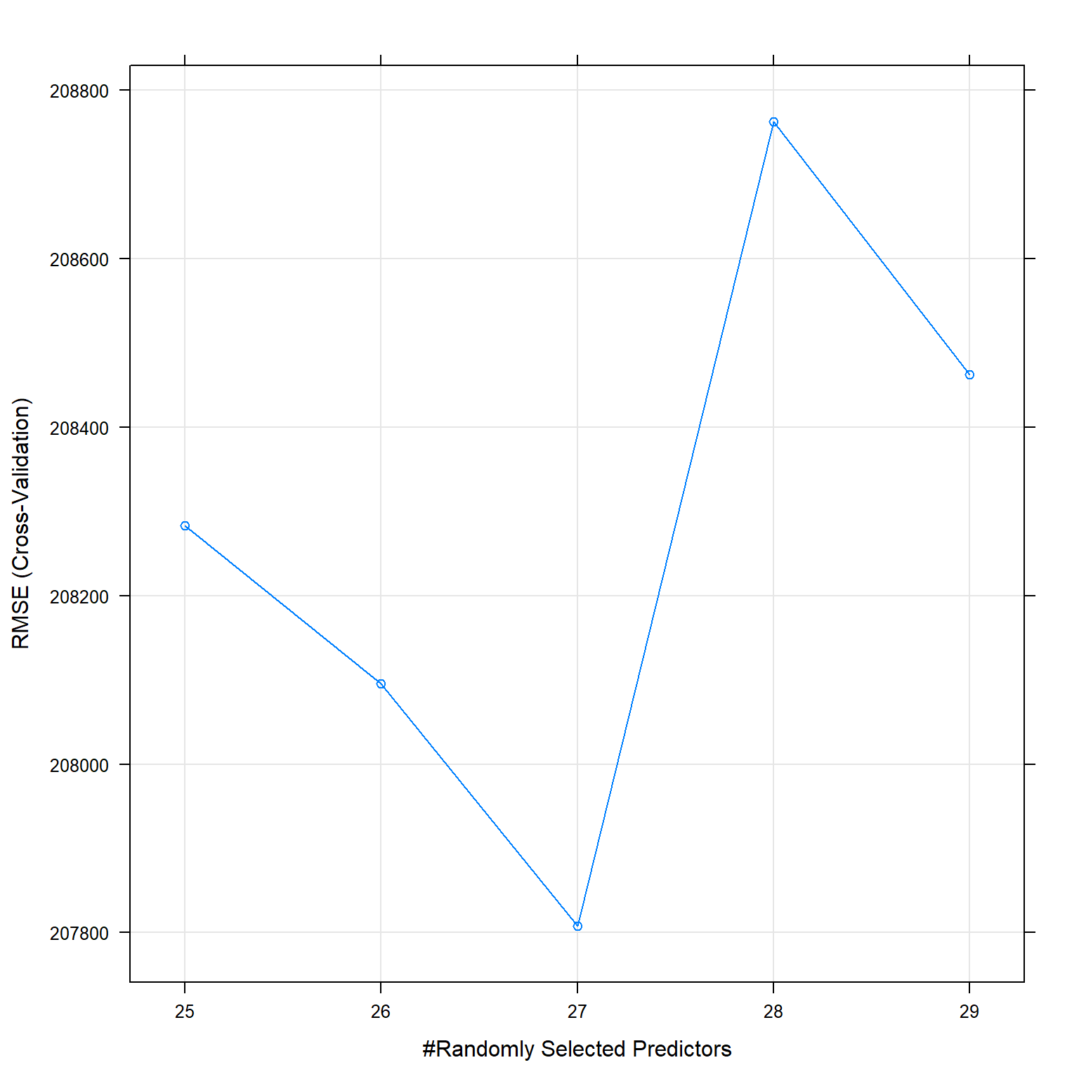
The best .mtry is 27.
Prediction RF
rf_prediction <- predict(rf_fit_2, newdata = test_data)

rf_results<-data.frame(RMSE = RMSE(rf_prediction, test_data$price), Rsquare = R2(rf_prediction, test_data$price))

rf_results
## RMSE Rsquare
## 1 194590 0.855Gradient Boosting Machine
Also gradient boosting is an ensembled learning method based on trees. Gradient boosting method combines the current model with the next best possible model as long as the combined model presents a lower overall error (RMSE) than the individual model. To optimize RMSE and R², I tune the maximum nodes per tree and the number of trees. An increasing number of trees reduces the error but could lead to over-fitting and needs much computational power. In addition, the learning rate (shrinkage) and the minimum number of observations in tree’s terminal nodes could potentially be tuned. I used a slow learn rate of 0.05 as recommended when growing trees and due to the size of my training data, 10 as minimum number of observations.
modelLookup("gbm")

#Usual trainControl - take the same

#Expand the search grid (see above for definitions)
grid<-expand.grid(interaction.depth = seq(4, 8, by = 2), #2. interaction.depth (Maximum nodes per tree) - number of splits it has to perform on a tree (starting from a single node).
                  n.trees = seq(500, 1500, by = 500), #Number of trees (the number of gradient boosting iteration) i.e. N. Increasing N reduces the error on training set, but setting it too high may lead to over-fitting.
                  shrinkage =0.05, #It is considered as a learning rate.Shrinkage is commonly used in ridge regression where it reduces regression coefficients to zero and, thus, reduces the impact of potentially unstable regression coefficients. , Use a small shrinkage (slow learn rate) when growing many trees.
                  n.minobsinnode = 10)#the minimum number of observations in trees' terminal nodes. Set n.minobsinnode = 10. When working with small training samples it may be vital to lower this setting to five or even three.

set.seed(1)
#Train for gbm
gbmFit1 <- train(price~

    distance_to_station
    +latitude
    +longitude

    +freehold_or_leasehold

    +district
    +property_type
    +london_zone
    +total_floor_area
    +number_habitable_rooms

    +energy_consumption_potential
    +windows_energy_eff
    +co2_emissions_potential
    +water_company,

     train_data,

                 method = "gbm",
                 trControl = control,#same as for lm
                 tuneGrid =grid,
                   metric = "RMSE",
                 verbose = FALSE
                 )


print(gbmFit1)modelLookup("gbm")## model parameter label forReg forClass probModel
## 1 gbm n.trees # Boosting Iterations TRUE TRUE TRUE
## 2 gbm interaction.depth Max Tree Depth TRUE TRUE TRUE
## 3 gbm shrinkage Shrinkage TRUE TRUE TRUE
## 4 gbm n.minobsinnode Min. Terminal Node Size TRUE TRUE TRUE#Usual trainControl - take the same
#Expand the search grid (see above for definitions)
grid<-expand.grid(interaction.depth = 8,
n.trees = 1500,
shrinkage =0.05,
n.minobsinnode = 10)#the minimum number of observations in trees' terminal nodes. Set n.minobsinnode = 10. When working with small training samples it may be vital to lower this setting to five or even three.
set.seed(1)
#Train for gbm
gbmFit1 <- train(price~
distance_to_station
+latitude
+longitude
+freehold_or_leasehold
+district
+property_type
+london_zone
+total_floor_area
+number_habitable_rooms
+energy_consumption_potential
+windows_energy_eff
+co2_emissions_potential
+water_company,
train_data,
method = "gbm",
trControl = control,#same as for lm
tuneGrid =grid,
metric = "RMSE",
verbose = FALSE
)
print(gbmFit1)## Stochastic Gradient Boosting
##
## 10499 samples
## 13 predictor
##
## No pre-processing
## Resampling: Cross-Validated (10 fold)
## Summary of sample sizes: 9450, 9450, 9449, 9448, 9450, 9449, ...
## Resampling results:
##
## RMSE Rsquared MAE
## 210923 0.84 99060
##
## Tuning parameter 'n.trees' was held constant at a value of 1500
##
## Tuning parameter 'shrinkage' was held constant at a value of 0.05
##
## Tuning parameter 'n.minobsinnode' was held constant at a value of 10RMSE was used to select the optimal model using the smallest value. The final values used for the model were n.trees = 1500, interaction.depth = 8, shrinkage = 0.05 and n.minobsinnode = 10.
gbm_prediction <- predict(gbmFit1, newdata = test_data)

gbm_results<-data.frame(RMSE = RMSE(gbm_prediction, test_data$price), Rsquare = R2(gbm_prediction, test_data$price))

gbm_results
Perfomance of the model (in R²): - Training 0.8403008 - Testing 0.8472716 201039.8
Stacking
Finally, I combine all the models that I trained and make a final prediction based on the predictions of the individual models. This method is an ensembled learning method called stacking and usually outperforms all the individual models.
#number of folds in cross validation
CVfolds <- 5

#Define folds
set.seed(1)
  #create five folds with no repeats
indexPreds <- createMultiFolds(train_data$price, CVfolds,times = 1)
#Define traincontrol using folds
ctrl <- trainControl(method = "cv",  number = CVfolds, returnResamp = "final", savePredictions = "final", index = indexPreds,sampling = NULL)

#LINEAR REGRESSION
model_lm<-train(
    price ~
   num_tube_lines
   +distance_to_station

    +district:property_type
    +london_zone*poly(total_floor_area,2)*number_habitable_rooms

   +average_income

    +energy_consumption_potential
    +windows_energy_eff
    +co2_emissions_potential
    +water_company

    ,
    train_data,
   method = "lm",
    trControl = ctrl
   )

# LASSO
lasso_fit <- train(price ~

   num_tube_lines
   +distance_to_station

    +district:property_type
    +london_zone*poly(total_floor_area,2)*number_habitable_rooms

   +average_income

    +energy_consumption_potential
    +windows_energy_eff
    +co2_emissions_potential
    +water_company,

        data=train_data,
        method="glmnet",
        preProc = c("center", "scale"), #This option standardizes the data before running the LASSO regression if alpha = 0 ->RIDGE REG

   trControl = ctrl,
  tuneGrid = expand.grid(alpha = 1, lambda = 40.40404) #insert the optimized
)

# TREE
model_tree_2 <- train(
  price ~

   num_tube_lines

    +latitude
    +longitude

    +district
    +property_type
    +london_zone
    +total_floor_area
    +number_habitable_rooms
    +average_income

    +energy_consumption_potential
    +windows_energy_eff
    +co2_emissions_potential
    +water_company
  ,
  train_data,

  method = "rpart",
  metric="RMSE",
  trControl = ctrl,
  tuneGrid= expand.grid(cp=0.00002)
    )

#KNN

knn_fit_2 <- train(
  price ~

   num_tube_lines

    +latitude
    +longitude

    +district
    +property_type
    +london_zone
    +total_floor_area
    +number_habitable_rooms
    +average_income

    +energy_consumption_potential
    +windows_energy_eff
    +co2_emissions_potential
    +water_company
  ,
  train_data,

    method = "knn",
     trControl = ctrl,
     tuneGrid = expand.grid(k=6), #looking for numbers around
     preProcess = c("center", "scale"), #center and scale the data in k-nn this is pretty important
     metric="RMSE") #default metric is accuracy is binary, otherwise RMSE, I change it to R²


# Random Forest
rf_fit_2 <- train(price~

   distance_to_station
   +latitude
   +longitude


   +freehold_or_leasehold

   +district
   +property_type
   +london_zone
   +total_floor_area
   +number_habitable_rooms

   +energy_consumption_potential
   +windows_energy_eff
   +co2_emissions_potential
   +water_company,

    train_data,

    method = "ranger",
    metric="RMSE",
    trControl = ctrl,
    tuneGrid = data.frame(.mtry = 27, .splitrule="variance", .min.node.size = 5),
    importance = 'permutation')


# Gradient
grid<-expand.grid(interaction.depth = 8, #seq(6, 10, by = 2), #2. interaction.depth (Maximum nodes per tree) - number of splits it has to perform on a tree (starting from a single node).
                  n.trees = 1500,##Number of trees (the number of gradient boosting iteration) i.e. N. Increasing N reduces the error on training set, but setting it too high may lead to over-fitting.
                  shrinkage =0.05, #It is considered as a learning rate, use a small shrinkage (slow learn rate) when growing many trees.
                  n.minobsinnode = 10)#the minimum number of observations in trees' terminal nodes.

gbmFit1 <- train(price~

    distance_to_station
    +latitude
    +longitude

    +freehold_or_leasehold

    +district
    +property_type
    +london_zone
    +total_floor_area
    +number_habitable_rooms

    +energy_consumption_potential
    +windows_energy_eff
    +co2_emissions_potential
    +water_company,

     train_data,

                 method = "gbm",
                 trControl = ctrl,
                 tuneGrid =grid,
                   metric = "RMSE"
                 )
## Iter TrainDeviance ValidDeviance StepSize Improve
## 1 247437688705.4287 nan 0.0500 16801252301.2286
## 2 232000278268.7830 nan 0.0500 15690971801.8620
## 3 218828715591.3823 nan 0.0500 14106227202.8752
## 4 205149091076.5482 nan 0.0500 12788910307.6939
## 5 193468845035.5358 nan 0.0500 9757749739.6899
## 6 183062089130.4374 nan 0.0500 10848202067.8948
## 7 172291539975.4364 nan 0.0500 9470000832.9087
## 8 163214068742.9066 nan 0.0500 7615975344.3065
## 9 154737960754.7700 nan 0.0500 7875555203.9193
## 10 147833823108.9143 nan 0.0500 7109522111.4091
## 20 95624937375.2434 nan 0.0500 2488688721.7182
## 40 58092570913.3721 nan 0.0500 950912601.8645
## 60 45720667173.3667 nan 0.0500 216688799.9767
## 80 40422896772.1081 nan 0.0500 137066553.2981
## 100 37088400609.1000 nan 0.0500 -80460469.0406
## 120 34632966244.9075 nan 0.0500 -120556986.8314
## 140 32705038931.6038 nan 0.0500 -82286260.6530
## 160 31108822663.6984 nan 0.0500 -50359260.6044
## 180 29804648110.2538 nan 0.0500 -45773553.0638
## 200 28475772744.5148 nan 0.0500 -61852314.9401
## 220 27377462100.7449 nan 0.0500 -47809341.3956
## 240 26490908447.8670 nan 0.0500 -128925155.8264
## 260 25556126149.4352 nan 0.0500 -19549531.7794
## 280 24635458756.1371 nan 0.0500 -78076118.9399
## 300 23948105351.6986 nan 0.0500 -38316972.5993
## 320 23272549122.9257 nan 0.0500 -33706969.5887
## 340 22490097524.4572 nan 0.0500 -59175625.4364
## 360 21913320289.2327 nan 0.0500 -81212438.8221
## 380 21274755158.0386 nan 0.0500 -36026982.3494
## 400 20599748547.6230 nan 0.0500 -14355642.3414
## 420 20068631707.7723 nan 0.0500 -12469755.2147
## 440 19542858228.6832 nan 0.0500 -11172592.0571
## 460 18957357908.1856 nan 0.0500 -30209488.4526
## 480 18520113900.8436 nan 0.0500 -44097434.8410
## 500 18106351966.9998 nan 0.0500 -2689730.3581
## 520 17729385466.6864 nan 0.0500 -23576089.0579
## 540 17364459474.5803 nan 0.0500 -23042515.0439
## 560 16993376893.4093 nan 0.0500 -26829867.2448
## 580 16637945433.6468 nan 0.0500 -5031381.5125
## 600 16241509125.1088 nan 0.0500 -28517106.0280
## 620 15949782148.7863 nan 0.0500 -19627916.7605
## 640 15644076619.6955 nan 0.0500 -19562244.3131
## 660 15367835705.5778 nan 0.0500 -32529324.8970
## 680 15121015306.8522 nan 0.0500 -6995581.9433
## 700 14829581815.4196 nan 0.0500 12299534.4644
## 720 14584374758.2405 nan 0.0500 -18207259.6416
## 740 14361383025.5789 nan 0.0500 -10153063.1291
## 760 14113383270.6949 nan 0.0500 -2342932.3574
## 780 13859412434.8414 nan 0.0500 -21503185.5878
## 800 13608157151.5257 nan 0.0500 -17122922.7747
## 820 13405498629.3242 nan 0.0500 -11937472.9078
## 840 13194032278.9143 nan 0.0500 -29046910.0443
## 860 12991025036.5170 nan 0.0500 -12257807.3376
## 880 12772064407.5574 nan 0.0500 -4436759.1798
## 900 12605245762.4946 nan 0.0500 -2316528.2865
## 920 12436950735.2306 nan 0.0500 -5876477.6883
## 940 12248571760.3645 nan 0.0500 -4719345.9821
## 960 12071145325.9307 nan 0.0500 -8056584.7381
## 980 11872934646.7866 nan 0.0500 -12635342.6009
## 1000 11691570997.7380 nan 0.0500 -12517932.8066
## 1020 11533281478.7139 nan 0.0500 -11155896.7995
## 1040 11358480874.8904 nan 0.0500 -7089073.4319
## 1060 11233333550.3298 nan 0.0500 -9573067.8657
## 1080 11087773656.8590 nan 0.0500 -11676314.5897
## 1100 10939282478.3953 nan 0.0500 -10325639.8591
## 1120 10806951942.8404 nan 0.0500 -10566758.2213
## 1140 10673602322.8670 nan 0.0500 -8394480.4835
## 1160 10532386780.4276 nan 0.0500 -12659095.1066
## 1180 10388414557.8044 nan 0.0500 5537969.6325
## 1200 10267046954.5759 nan 0.0500 -5298494.5268
## 1220 10138555309.0737 nan 0.0500 -1417217.0564
## 1240 10007393587.1272 nan 0.0500 -7221218.4085
## 1260 9884409148.0953 nan 0.0500 -3893119.3180
## 1280 9766316088.5224 nan 0.0500 -6982833.8691
## 1300 9641018051.4913 nan 0.0500 -6058292.3689
## 1320 9525771025.4948 nan 0.0500 -13425171.2655
## 1340 9428161845.2522 nan 0.0500 -12974105.7873
## 1360 9310307904.4361 nan 0.0500 -4800012.5692
## 1380 9197895335.2128 nan 0.0500 -5212347.4768
## 1400 9095293289.4673 nan 0.0500 -11650171.7175
## 1420 8985995031.2347 nan 0.0500 2916449.3046
## 1440 8885559645.2912 nan 0.0500 -7129216.5155
## 1460 8790457619.8345 nan 0.0500 -9212977.3824
## 1480 8696663815.7667 nan 0.0500 -6896679.9748
## 1500 8597522170.1863 nan 0.0500 -6298537.6785
##
## Iter TrainDeviance ValidDeviance StepSize Improve
## 1 251203392392.6218 nan 0.0500 19344882605.9957
## 2 234529263549.3858 nan 0.0500 17483443616.1385
## 3 220173872432.6830 nan 0.0500 14467723251.8060
## 4 206328159598.5661 nan 0.0500 11265029035.4564
## 5 194161485143.1612 nan 0.0500 10743208848.0867
## 6 183708627434.2637 nan 0.0500 10668275198.3186
## 7 173237403545.4839 nan 0.0500 10336632424.6296
## 8 164298076597.5103 nan 0.0500 7780511081.7556
## 9 155792614724.3971 nan 0.0500 7173932923.2228
## 10 148457780399.1842 nan 0.0500 6910057664.0994
## 20 97763732035.2382 nan 0.0500 2875515430.3423
## 40 58900773855.1187 nan 0.0500 918231443.3753
## 60 46183142670.6044 nan 0.0500 253414611.3341
## 80 40201278078.0805 nan 0.0500 69071359.8496
## 100 36699451908.0091 nan 0.0500 -4516673.3067
## 120 34302018774.7417 nan 0.0500 -9793333.4514
## 140 32239454530.4458 nan 0.0500 -35196531.9144
## 160 30903961176.0136 nan 0.0500 -107953654.9803
## 180 29609868801.4378 nan 0.0500 11564621.6200
## 200 28272624249.7456 nan 0.0500 42234699.3563
## 220 27215128104.3425 nan 0.0500 -38628780.3761
## 240 26227552075.7280 nan 0.0500 -36024153.9477
## 260 25382314915.9630 nan 0.0500 5581784.5762
## 280 24558449616.3890 nan 0.0500 -17399545.5599
## 300 23800143557.5414 nan 0.0500 -28672447.0224
## 320 23228259880.5985 nan 0.0500 -17536645.3697
## 340 22611033158.6527 nan 0.0500 -39774918.4282
## 360 22140754789.0262 nan 0.0500 -29909985.4045
## 380 21539089965.2597 nan 0.0500 -56837071.4607
## 400 21006010445.1879 nan 0.0500 -19866737.5342
## 420 20570501692.2485 nan 0.0500 -29590002.3431
## 440 20127696884.5072 nan 0.0500 -45831246.8909
## 460 19655207296.3137 nan 0.0500 -20441181.9312
## 480 19241343967.6648 nan 0.0500 -26365636.8724
## 500 18832311092.0197 nan 0.0500 -45451824.1377
## 520 18316443033.3673 nan 0.0500 -60991947.8298
## 540 17919126655.5172 nan 0.0500 -14575932.5523
## 560 17578663913.5246 nan 0.0500 -22899199.9812
## 580 17232961523.5101 nan 0.0500 -30097122.0064
## 600 16889764649.2289 nan 0.0500 -12629884.3628
## 620 16578600806.3272 nan 0.0500 -13320013.4055
## 640 16304986461.5123 nan 0.0500 -6501267.9757
## 660 16005890114.1592 nan 0.0500 -18230020.6700
## 680 15686469037.5680 nan 0.0500 -46999612.9232
## 700 15403856111.9631 nan 0.0500 -27166298.6348
## 720 15127514481.1521 nan 0.0500 -24820471.2971
## 740 14852155115.9459 nan 0.0500 -16084368.7082
## 760 14568011376.2146 nan 0.0500 -19219897.0704
## 780 14294724529.1704 nan 0.0500 9065125.2962
## 800 14023171519.7364 nan 0.0500 -26434488.8656
## 820 13819591704.6066 nan 0.0500 -18162991.4190
## 840 13591781834.2017 nan 0.0500 -20190265.1968
## 860 13382386123.3599 nan 0.0500 -4419774.3000
## 880 13175049039.0262 nan 0.0500 -18230969.3747
## 900 12981550883.2149 nan 0.0500 -16212708.1816
## 920 12774177215.8483 nan 0.0500 -12548070.3101
## 940 12584930645.3376 nan 0.0500 -8206728.6178
## 960 12406856216.8821 nan 0.0500 -17873884.2780
## 980 12208764478.9520 nan 0.0500 4002501.3718
## 1000 12041402422.3606 nan 0.0500 -15007376.5228
## 1020 11888619859.1288 nan 0.0500 -10304794.2639
## 1040 11729419641.1294 nan 0.0500 -7997410.8868
## 1060 11552969034.2644 nan 0.0500 -1060328.2748
## 1080 11398003761.4592 nan 0.0500 -16261175.9755
## 1100 11243669602.3688 nan 0.0500 -654272.8387
## 1120 11107895547.1591 nan 0.0500 -14972216.5820
## 1140 10992705728.9962 nan 0.0500 -3329225.7788
## 1160 10850873737.8402 nan 0.0500 -17387176.9088
## 1180 10719762185.4472 nan 0.0500 -18864670.8849
## 1200 10581010520.8986 nan 0.0500 -3139779.3311
## 1220 10436798609.9160 nan 0.0500 -18672376.0004
## 1240 10322270295.5927 nan 0.0500 -14248382.3870
## 1260 10188391548.8068 nan 0.0500 4382505.7696
## 1280 10052155777.3462 nan 0.0500 -1733655.9220
## 1300 9938786238.2663 nan 0.0500 3050129.0254
## 1320 9822575226.6972 nan 0.0500 -11962581.4963
## 1340 9711724050.8268 nan 0.0500 -11770566.6723
## 1360 9587038187.6770 nan 0.0500 -822333.6319
## 1380 9488740978.3182 nan 0.0500 -6620612.3834
## 1400 9383516481.3260 nan 0.0500 -9789046.0878
## 1420 9267603771.8339 nan 0.0500 -340856.8886
## 1440 9166119635.1323 nan 0.0500 -11159009.6714
## 1460 9067276906.2260 nan 0.0500 -79573.5737
## 1480 8969042475.5866 nan 0.0500 -4810129.8591
## 1500 8876747816.7409 nan 0.0500 1258214.5088
##
## Iter TrainDeviance ValidDeviance StepSize Improve
## 1 257832453782.5124 nan 0.0500 19602069228.8723
## 2 241082847214.0711 nan 0.0500 18014915801.4955
## 3 226147129184.6718 nan 0.0500 15610551148.6476
## 4 212483943930.3416 nan 0.0500 14120372400.8190
## 5 200290053366.6906 nan 0.0500 12807336022.7842
## 6 188683691101.6127 nan 0.0500 9697859385.7568
## 7 177055708949.3166 nan 0.0500 11286524552.0228
## 8 167361969167.4400 nan 0.0500 9084676439.0758
## 9 158245404946.2050 nan 0.0500 8411053317.3486
## 10 149852517903.2663 nan 0.0500 7286703276.9721
## 20 95932971388.8225 nan 0.0500 3872198582.6725
## 40 57469358375.5171 nan 0.0500 859251216.6947
## 60 44132083337.5622 nan 0.0500 -45260808.1626
## 80 38734596859.0976 nan 0.0500 42685945.9327
## 100 35783232325.8149 nan 0.0500 -59407880.7167
## 120 33534472681.1316 nan 0.0500 -90182502.5801
## 140 31670865299.9807 nan 0.0500 30693393.0432
## 160 30399762830.5174 nan 0.0500 -75498694.2365
## 180 29053507112.1285 nan 0.0500 -32876814.1289
## 200 27660526988.9776 nan 0.0500 -59604574.9750
## 220 26661881812.8947 nan 0.0500 -44880190.4880
## 240 25805513127.7589 nan 0.0500 -34775555.9173
## 260 24951058150.6592 nan 0.0500 -38280813.8107
## 280 24265190184.7988 nan 0.0500 -89865069.2265
## 300 23514899191.8895 nan 0.0500 -55939094.2960
## 320 22846529489.5833 nan 0.0500 -21678901.5008
## 340 22241722931.6147 nan 0.0500 -72639543.4436
## 360 21669254450.4368 nan 0.0500 -50194359.9988
## 380 21071626810.0067 nan 0.0500 -68234595.7483
## 400 20669073172.2180 nan 0.0500 742271.2956
## 420 20198969016.0675 nan 0.0500 -30482270.8289
## 440 19701711111.2000 nan 0.0500 -13790515.0276
## 460 19277684929.6747 nan 0.0500 -17597674.2445
## 480 18851986432.5235 nan 0.0500 -30658769.2931
## 500 18419872309.0325 nan 0.0500 -12709707.5661
## 520 18034503236.8089 nan 0.0500 -2652920.0498
## 540 17669477555.0583 nan 0.0500 -18499678.1658
## 560 17323280148.1029 nan 0.0500 -6389876.5418
## 580 17002830888.6033 nan 0.0500 -11224128.3790
## 600 16687777520.3583 nan 0.0500 -27055275.9887
## 620 16385256636.7353 nan 0.0500 -4810463.7090
## 640 16071995743.3280 nan 0.0500 -17698091.0570
## 660 15807069050.6145 nan 0.0500 -14777260.5033
## 680 15507406014.9158 nan 0.0500 -31272771.7744
## 700 15218299674.2426 nan 0.0500 -20817229.4336
## 720 14972368172.4079 nan 0.0500 -36049140.5975
## 740 14734570617.9544 nan 0.0500 -20105028.3027
## 760 14460319326.3111 nan 0.0500 -6387907.1781
## 780 14211407588.8203 nan 0.0500 3711776.9274
## 800 13961047159.7350 nan 0.0500 -24287686.6757
## 820 13744819908.1639 nan 0.0500 3170680.0159
## 840 13477364031.8947 nan 0.0500 -28227326.6305
## 860 13263240331.5939 nan 0.0500 -15065353.7046
## 880 13082541088.3425 nan 0.0500 -16028019.4990
## 900 12902809225.5303 nan 0.0500 -23779974.8605
## 920 12724318288.2856 nan 0.0500 -3147657.2575
## 940 12539307152.1351 nan 0.0500 -3654384.6394
## 960 12335050319.1319 nan 0.0500 -14443040.5316
## 980 12168639840.8320 nan 0.0500 -14977260.9678
## 1000 11996209100.4582 nan 0.0500 -18693892.2972
## 1020 11855901659.7468 nan 0.0500 -8798645.8295
## 1040 11699581425.6238 nan 0.0500 -15970362.9078
## 1060 11539082468.2978 nan 0.0500 2981656.5609
## 1080 11394951775.2452 nan 0.0500 -13174392.2152
## 1100 11235164367.1390 nan 0.0500 -5736375.9502
## 1120 11106895481.5597 nan 0.0500 -10727736.8546
## 1140 10942314463.4981 nan 0.0500 -12364184.2845
## 1160 10803770740.9620 nan 0.0500 -4580430.6311
## 1180 10679405648.8745 nan 0.0500 3395139.3460
## 1200 10570311415.0426 nan 0.0500 -19403432.6361
## 1220 10442359059.4609 nan 0.0500 -4806954.1705
## 1240 10291586634.7517 nan 0.0500 -3595122.0516
## 1260 10160402194.9309 nan 0.0500 806074.6402
## 1280 10035462951.9658 nan 0.0500 -3462910.6448
## 1300 9902785388.8658 nan 0.0500 8891951.5147
## 1320 9783589863.5066 nan 0.0500 -8452873.1774
## 1340 9657263218.3910 nan 0.0500 -6885831.0535
## 1360 9547039887.5819 nan 0.0500 -9991172.5045
## 1380 9431280498.4185 nan 0.0500 -6288002.1895
## 1400 9322022219.2580 nan 0.0500 -9258141.5213
## 1420 9223275930.6152 nan 0.0500 -8740198.1921
## 1440 9120383844.6298 nan 0.0500 -11226898.1740
## 1460 9009490297.2610 nan 0.0500 -1332762.9914
## 1480 8915281768.0753 nan 0.0500 2071345.6554
## 1500 8822700901.2461 nan 0.0500 -8519650.6575
##
## Iter TrainDeviance ValidDeviance StepSize Improve
## 1 258768875615.4841 nan 0.0500 20788264223.2576
## 2 242298274267.3581 nan 0.0500 16189472667.0661
## 3 227263309703.9819 nan 0.0500 15607427543.3734
## 4 213562699686.1152 nan 0.0500 12810910203.6035
## 5 200583642217.8555 nan 0.0500 12715454695.3170
## 6 188612312716.7159 nan 0.0500 9291512107.7753
## 7 177815681232.6924 nan 0.0500 8854729872.0179
## 8 168707280715.0586 nan 0.0500 9448714372.1164
## 9 160327643564.3338 nan 0.0500 9304522755.6371
## 10 152052729079.2238 nan 0.0500 7285335039.3477
## 20 99277880132.5523 nan 0.0500 3525041391.9227
## 40 59075420404.3493 nan 0.0500 758098076.2381
## 60 45905132944.3801 nan 0.0500 150864832.3737
## 80 40277765243.4037 nan 0.0500 27085350.5500
## 100 37252416978.5639 nan 0.0500 -29250723.9635
## 120 34915631799.6153 nan 0.0500 -80017300.3011
## 140 32887470759.3464 nan 0.0500 -74906855.3093
## 160 31401257065.3274 nan 0.0500 -27781236.9718
## 180 30008414301.3661 nan 0.0500 -54407669.8603
## 200 28995391616.5640 nan 0.0500 -38983037.9838
## 220 27992351945.6012 nan 0.0500 -54059565.1321
## 240 27094069813.1610 nan 0.0500 -25595973.8679
## 260 26056645515.6979 nan 0.0500 -39778018.3336
## 280 25106734311.1263 nan 0.0500 -8148969.1881
## 300 24401721846.3725 nan 0.0500 -31716119.1427
## 320 23592250736.3010 nan 0.0500 -24536548.2942
## 340 22819019757.0565 nan 0.0500 21452978.2207
## 360 22235140028.0625 nan 0.0500 -42580206.8320
## 380 21650235391.2817 nan 0.0500 -23121481.4526
## 400 21147917667.8512 nan 0.0500 -40850834.1961
## 420 20649394224.4801 nan 0.0500 -55632730.6568
## 440 20164827285.9685 nan 0.0500 -34340111.6986
## 460 19708008366.1965 nan 0.0500 -26904900.6645
## 480 19163493100.6559 nan 0.0500 11462885.8101
## 500 18762139710.6187 nan 0.0500 -27961580.6964
## 520 18248676146.9786 nan 0.0500 -36589403.1521
## 540 17865487362.6215 nan 0.0500 -5754457.7977
## 560 17442198203.4223 nan 0.0500 -17487433.4555
## 580 17092016004.5553 nan 0.0500 -31181480.5679
## 600 16778577401.1917 nan 0.0500 -26402570.4252
## 620 16418756018.0820 nan 0.0500 -2622766.7861
## 640 16155299955.4977 nan 0.0500 -28190448.2910
## 660 15852122475.1059 nan 0.0500 -16868453.1137
## 680 15575640034.9584 nan 0.0500 -15345975.5106
## 700 15324115238.3178 nan 0.0500 -12851562.0436
## 720 15110786147.6783 nan 0.0500 -17310284.7596
## 740 14853194945.5165 nan 0.0500 -7848858.8144
## 760 14614309703.2426 nan 0.0500 -17807954.1999
## 780 14369559183.0986 nan 0.0500 -12510305.6648
## 800 14092528357.5526 nan 0.0500 -6374997.2305
## 820 13873968825.9696 nan 0.0500 -11252037.1803
## 840 13682949620.5290 nan 0.0500 345197.7131
## 860 13463736144.5008 nan 0.0500 -11103568.2348
## 880 13277150862.4057 nan 0.0500 -20943408.6402
## 900 13041187565.4077 nan 0.0500 3852015.0117
## 920 12839575609.2895 nan 0.0500 -11925749.6978
## 940 12629135530.9884 nan 0.0500 -12482762.9303
## 960 12445795992.2094 nan 0.0500 -9646217.7820
## 980 12260808708.5173 nan 0.0500 -15758908.5782
## 1000 12083464020.0268 nan 0.0500 -9510428.8467
## 1020 11895993728.2972 nan 0.0500 -3224239.8537
## 1040 11736551883.0273 nan 0.0500 -8985759.7424
## 1060 11560260419.9724 nan 0.0500 -17368129.0168
## 1080 11395890559.5762 nan 0.0500 -11636344.5716
## 1100 11231462960.8721 nan 0.0500 -9201865.8273
## 1120 11095110727.1141 nan 0.0500 4321402.4205
## 1140 10956612229.8037 nan 0.0500 -16920348.8914
## 1160 10817810555.9859 nan 0.0500 -8250178.0734
## 1180 10686306953.7374 nan 0.0500 -16032329.7398
## 1200 10548078737.6017 nan 0.0500 -1641263.5025
## 1220 10416379858.2776 nan 0.0500 -10226178.8852
## 1240 10296831939.4207 nan 0.0500 -7050287.6795
## 1260 10182730595.6681 nan 0.0500 -5787638.6946
## 1280 10055694115.5930 nan 0.0500 -5402335.5294
## 1300 9930160381.4398 nan 0.0500 -11579779.3864
## 1320 9807854130.5481 nan 0.0500 -8008083.5546
## 1340 9717342106.8317 nan 0.0500 -14565342.7346
## 1360 9611239891.0548 nan 0.0500 1316366.7541
## 1380 9500817498.2141 nan 0.0500 -1069072.8462
## 1400 9415000376.5840 nan 0.0500 -1209869.0486
## 1420 9314737734.9074 nan 0.0500 -5298688.6195
## 1440 9220758829.8052 nan 0.0500 -11794477.6778
## 1460 9123231821.6435 nan 0.0500 -8354817.5872
## 1480 9024711307.9251 nan 0.0500 -19240373.8671
## 1500 8920470232.8748 nan 0.0500 -6467160.5776
##
## Iter TrainDeviance ValidDeviance StepSize Improve
## 1 258909339918.8690 nan 0.0500 18844999337.4506
## 2 243891483172.0254 nan 0.0500 15078073696.5793
## 3 229591388437.0222 nan 0.0500 12956388217.6491
## 4 215024474771.6006 nan 0.0500 15502393800.4451
## 5 202976870668.8875 nan 0.0500 13618598007.9925
## 6 192131546117.8822 nan 0.0500 10726006952.1989
## 7 181814208454.6968 nan 0.0500 10066577822.1216
## 8 172262606644.6008 nan 0.0500 9347443783.6331
## 9 163401508866.7413 nan 0.0500 9269358684.6585
## 10 154624664126.8134 nan 0.0500 8049065044.0284
## 20 100380384229.5783 nan 0.0500 3535429361.4723
## 40 58787923181.1791 nan 0.0500 633834165.9540
## 60 45226458906.7937 nan 0.0500 293888167.3495
## 80 39951415652.9891 nan 0.0500 -22940656.4192
## 100 36855600725.6866 nan 0.0500 -196595541.1954
## 120 34258667364.7127 nan 0.0500 -92221266.9923
## 140 32210515254.2621 nan 0.0500 -16944888.6598
## 160 30568807494.8040 nan 0.0500 -82288389.1737
## 180 29064076672.0278 nan 0.0500 -96274393.4498
## 200 27792900937.6425 nan 0.0500 -49455106.5358
## 220 26588756829.0611 nan 0.0500 -57142617.5414
## 240 25519894899.6631 nan 0.0500 -95028649.7053
## 260 24494794405.7692 nan 0.0500 -56032097.4869
## 280 23732351364.7546 nan 0.0500 -59850140.7348
## 300 23042201593.4881 nan 0.0500 -28454664.9745
## 320 22328019599.3422 nan 0.0500 -55136947.5459
## 340 21581907236.1899 nan 0.0500 -25208196.8429
## 360 20939722023.3211 nan 0.0500 -22806351.2030
## 380 20348132864.2421 nan 0.0500 -25897418.2975
## 400 19867626719.8213 nan 0.0500 -51518384.1216
## 420 19339397599.9123 nan 0.0500 1981498.5579
## 440 18893382630.2561 nan 0.0500 -30185496.9763
## 460 18454067362.9378 nan 0.0500 1701148.0979
## 480 18052457201.8958 nan 0.0500 -18003665.3678
## 500 17618309814.1054 nan 0.0500 -32596938.6268
## 520 17225763925.7692 nan 0.0500 -12783373.4203
## 540 16872406732.2674 nan 0.0500 -34156346.3204
## 560 16567314977.6310 nan 0.0500 -13774437.4431
## 580 16234993611.0253 nan 0.0500 -5251047.4825
## 600 15895991653.8401 nan 0.0500 -28171362.0151
## 620 15576906468.9031 nan 0.0500 -6249888.8830
## 640 15284718113.8470 nan 0.0500 -19379694.2935
## 660 14972057047.7235 nan 0.0500 -1297524.0640
## 680 14717157974.3155 nan 0.0500 -12022341.8302
## 700 14442294239.9017 nan 0.0500 -16836561.6537
## 720 14200901942.8578 nan 0.0500 -15692619.5557
## 740 13931803657.5258 nan 0.0500 -8677562.6867
## 760 13677331957.0521 nan 0.0500 -2594177.5133
## 780 13462495016.4761 nan 0.0500 -9975521.7596
## 800 13247003867.6707 nan 0.0500 -5867438.0628
## 820 13025909794.3190 nan 0.0500 3209899.8004
## 840 12830231174.3768 nan 0.0500 -2641002.0109
## 860 12633627472.2446 nan 0.0500 -4280496.4233
## 880 12471302227.5607 nan 0.0500 -7976938.1678
## 900 12275922232.6236 nan 0.0500 -115036.5489
## 920 12093343104.6787 nan 0.0500 -15011981.1700
## 940 11936987780.9866 nan 0.0500 -6111448.2191
## 960 11787014782.8474 nan 0.0500 -11467468.5610
## 980 11638467041.1413 nan 0.0500 -6987665.9372
## 1000 11475426528.5388 nan 0.0500 -17822682.1647
## 1020 11325521744.5253 nan 0.0500 -13978043.4160
## 1040 11162272668.8892 nan 0.0500 -2627996.8707
## 1060 10978886950.4393 nan 0.0500 -14897115.6624
## 1080 10820635107.8792 nan 0.0500 -4220121.8955
## 1100 10688247211.5504 nan 0.0500 -10470243.2729
## 1120 10555227235.7617 nan 0.0500 -3808133.0762
## 1140 10433006669.8847 nan 0.0500 -8005977.1351
## 1160 10321301887.8452 nan 0.0500 -13349388.6427
## 1180 10183031244.9192 nan 0.0500 -7734792.7876
## 1200 10071892216.8314 nan 0.0500 -9085863.0799
## 1220 9941231028.1395 nan 0.0500 -2587628.1854
## 1240 9829051266.5810 nan 0.0500 -6591424.2098
## 1260 9701752922.7926 nan 0.0500 -1366447.6359
## 1280 9590841384.2869 nan 0.0500 -2543759.8275
## 1300 9479209751.0747 nan 0.0500 -15792012.2073
## 1320 9359235283.2509 nan 0.0500 -33807.9187
## 1340 9246705188.1748 nan 0.0500 -3802791.4265
## 1360 9143149175.8891 nan 0.0500 -7896967.3225
## 1380 9037994879.4216 nan 0.0500 -3053550.2541
## 1400 8947764588.8148 nan 0.0500 -7862819.1870
## 1420 8849245916.7855 nan 0.0500 -2314903.7042
## 1440 8767298474.2565 nan 0.0500 -9934904.6934
## 1460 8658106336.2579 nan 0.0500 -3818158.6872
## 1480 8559464725.5251 nan 0.0500 -10247861.3962
## 1500 8462116142.4200 nan 0.0500 -177752.6975
##
## Iter TrainDeviance ValidDeviance StepSize Improve
## 1 254061589297.6797 nan 0.0500 16707467520.3205
## 2 237727876492.4179 nan 0.0500 16341916930.8013
## 3 223250792049.8754 nan 0.0500 13949844036.1071
## 4 210597930293.1893 nan 0.0500 12996577532.9726
## 5 198652192665.2593 nan 0.0500 11806650447.0869
## 6 186625546581.9215 nan 0.0500 10778725861.8742
## 7 176893152834.0851 nan 0.0500 8918958067.7665
## 8 166297679018.5577 nan 0.0500 9835802406.7236
## 9 157571619326.7144 nan 0.0500 8218010207.1319
## 10 149997070285.4969 nan 0.0500 7561139285.5028
## 20 96711863945.0235 nan 0.0500 3336591495.7178
## 40 57134800820.1563 nan 0.0500 921554483.9302
## 60 44518284490.6246 nan 0.0500 232751469.6994
## 80 38984317768.0901 nan 0.0500 64681869.7492
## 100 36037628840.8775 nan 0.0500 -15603862.1741
## 120 33893332248.7045 nan 0.0500 36574013.0376
## 140 32322552413.1837 nan 0.0500 14276389.9365
## 160 30939286279.4923 nan 0.0500 -33730113.9104
## 180 29775392412.7720 nan 0.0500 -97194805.1931
## 200 28663486991.3102 nan 0.0500 -3540365.6663
## 220 27700360966.8449 nan 0.0500 8748848.2965
## 240 26736155783.5938 nan 0.0500 -41201853.5041
## 260 25989916027.8502 nan 0.0500 -57744328.4367
## 280 25287119178.2563 nan 0.0500 -44412715.6066
## 300 24470943385.5846 nan 0.0500 -49963342.7560
## 320 23799857488.8041 nan 0.0500 -19067004.7585
## 340 23183169638.7120 nan 0.0500 -20477871.5461
## 360 22683072900.0236 nan 0.0500 -42506709.1344
## 380 22125128108.6084 nan 0.0500 -51340005.9311
## 400 21623948384.1186 nan 0.0500 -35473910.2428
## 420 21157446857.0273 nan 0.0500 -22753420.2709
## 440 20583118511.9698 nan 0.0500 -26880528.0392
## 460 20176683737.8660 nan 0.0500 -39577606.3761
## 480 19781244585.3747 nan 0.0500 -25837473.8527
## 500 19408666881.4744 nan 0.0500 -13570609.1997
## 520 19053558919.2727 nan 0.0500 -23920631.0353
## 540 18702947212.8924 nan 0.0500 -29762458.1933
## 560 18361135336.6851 nan 0.0500 -10106440.8142
## 580 18057533510.3451 nan 0.0500 -11185155.3344
## 600 17697920464.6967 nan 0.0500 -23962152.0447
## 620 17384044560.3564 nan 0.0500 -1980860.3223
## 640 17092813323.3172 nan 0.0500 3451863.4620
## 660 16826451520.8222 nan 0.0500 -12484111.8287
## 680 16526345530.6201 nan 0.0500 -12800386.9243
## 700 16273595849.4316 nan 0.0500 -15184608.6109
## 720 15999756545.5648 nan 0.0500 -2329555.7880
## 740 15700752700.1574 nan 0.0500 -13109842.7084
## 760 15442364264.2017 nan 0.0500 -21702209.2440
## 780 15152009205.9528 nan 0.0500 6648059.8984
## 800 14935381902.6730 nan 0.0500 -15800294.5268
## 820 14724355671.9934 nan 0.0500 -25300481.7705
## 840 14497642202.0234 nan 0.0500 -7246855.3086
## 860 14301229878.1407 nan 0.0500 -17235959.9812
## 880 14118342559.7032 nan 0.0500 -24505958.8202
## 900 13867825949.3564 nan 0.0500 -2146673.6135
## 920 13675825370.8646 nan 0.0500 -11339556.8270
## 940 13496316501.2680 nan 0.0500 -3193636.2969
## 960 13326734670.8289 nan 0.0500 -1182916.8065
## 980 13150610118.5390 nan 0.0500 -9339504.2453
## 1000 12980442027.6338 nan 0.0500 -7968451.5679
## 1020 12805816292.9469 nan 0.0500 -13006352.9698
## 1040 12642013291.1660 nan 0.0500 -1777712.7314
## 1060 12468608971.9994 nan 0.0500 -8613299.5845
## 1080 12311180917.6355 nan 0.0500 -14600521.8862
## 1100 12160230572.6988 nan 0.0500 -9682642.6602
## 1120 11987462775.5350 nan 0.0500 -12374557.2553
## 1140 11842061976.5453 nan 0.0500 -7026835.8001
## 1160 11710632738.8370 nan 0.0500 3810345.3085
## 1180 11568116271.3770 nan 0.0500 -8856220.3612
## 1200 11439690894.8156 nan 0.0500 -7870074.7704
## 1220 11289178575.9091 nan 0.0500 -6932127.5612
## 1240 11170197237.6925 nan 0.0500 -8821673.1030
## 1260 11036398698.8110 nan 0.0500 -13423092.0605
## 1280 10898335689.2964 nan 0.0500 -5092489.6338
## 1300 10774694486.7303 nan 0.0500 -3030104.0653
## 1320 10668773961.5829 nan 0.0500 -9842026.1921
## 1340 10549785829.0096 nan 0.0500 -7735773.5874
## 1360 10431741671.0151 nan 0.0500 -11927802.4062
## 1380 10328873683.4323 nan 0.0500 -780244.1208
## 1400 10230866002.6588 nan 0.0500 -9649780.4170
## 1420 10132219931.3737 nan 0.0500 -6574881.4469
## 1440 10033889257.0840 nan 0.0500 -2939305.4942
## 1460 9935996593.9181 nan 0.0500 679091.0797
## 1480 9849385202.6572 nan 0.0500 -10371527.3147
## 1500 9756616797.8631 nan 0.0500 -7318059.3543#combine the results
#make sure to use the method names from above
multimodel <- list(
lm = model_lm,
gbm = gbmFit1,
knn=knn_fit_2,
glmnet=lasso_fit,
rpart = model_tree_2,
ramger =rf_fit_2
)
class(multimodel) <- "caretList"The figures below compare the 6 models used for stacking visually in terms of RMSE and R².
#we can visualize the differences in performance of each algorithm for each fold
dotplot(resamples(multimodel), metric = "Rsquared") #you can set metric=MAE, RMSE, or Rsquared 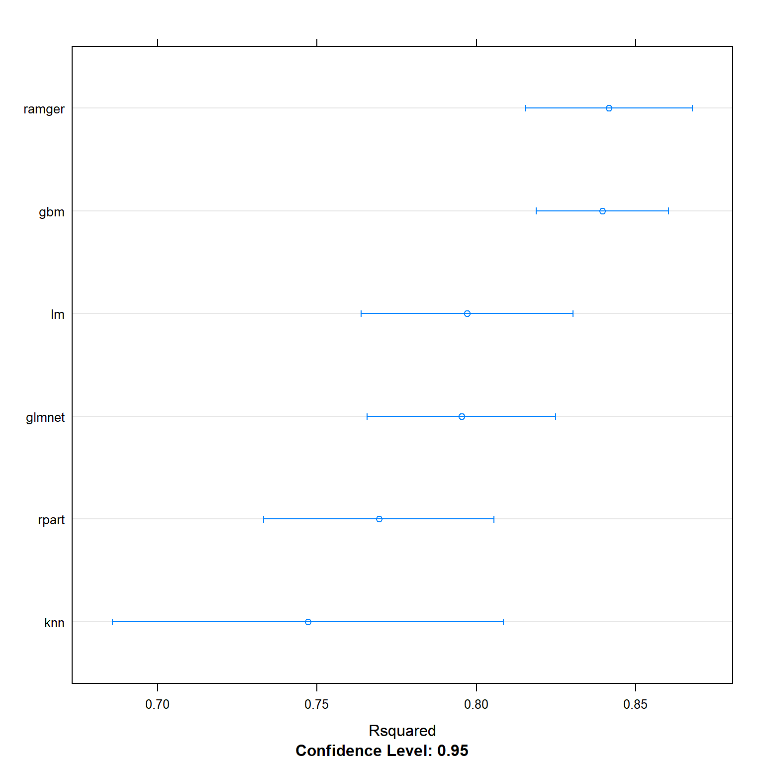
splom(resamples(multimodel), metric = "Rsquared")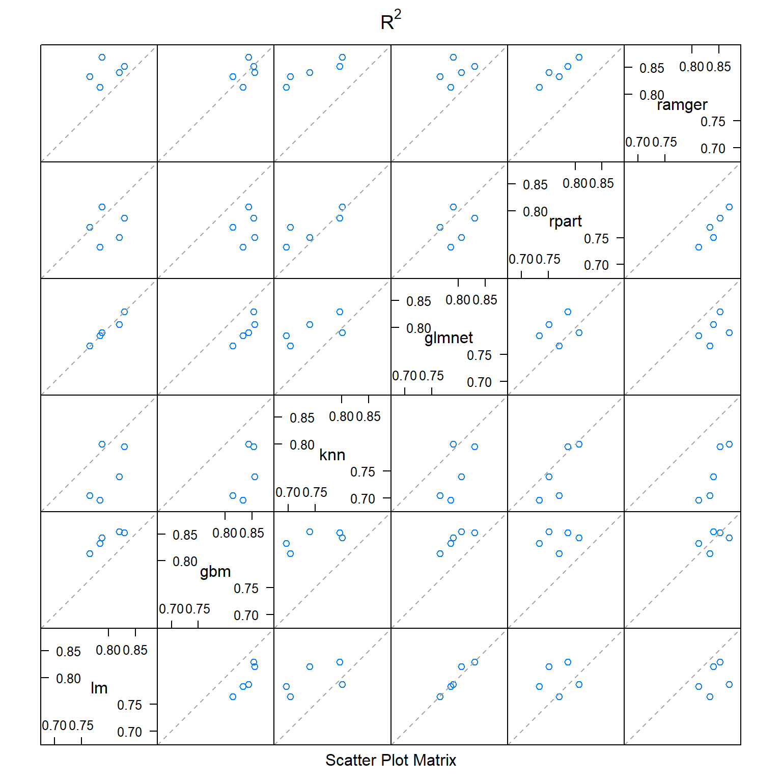
dotplot(resamples(multimodel), metric = "RMSE") #you can set metric=MAE, RMSE, or Rsquared 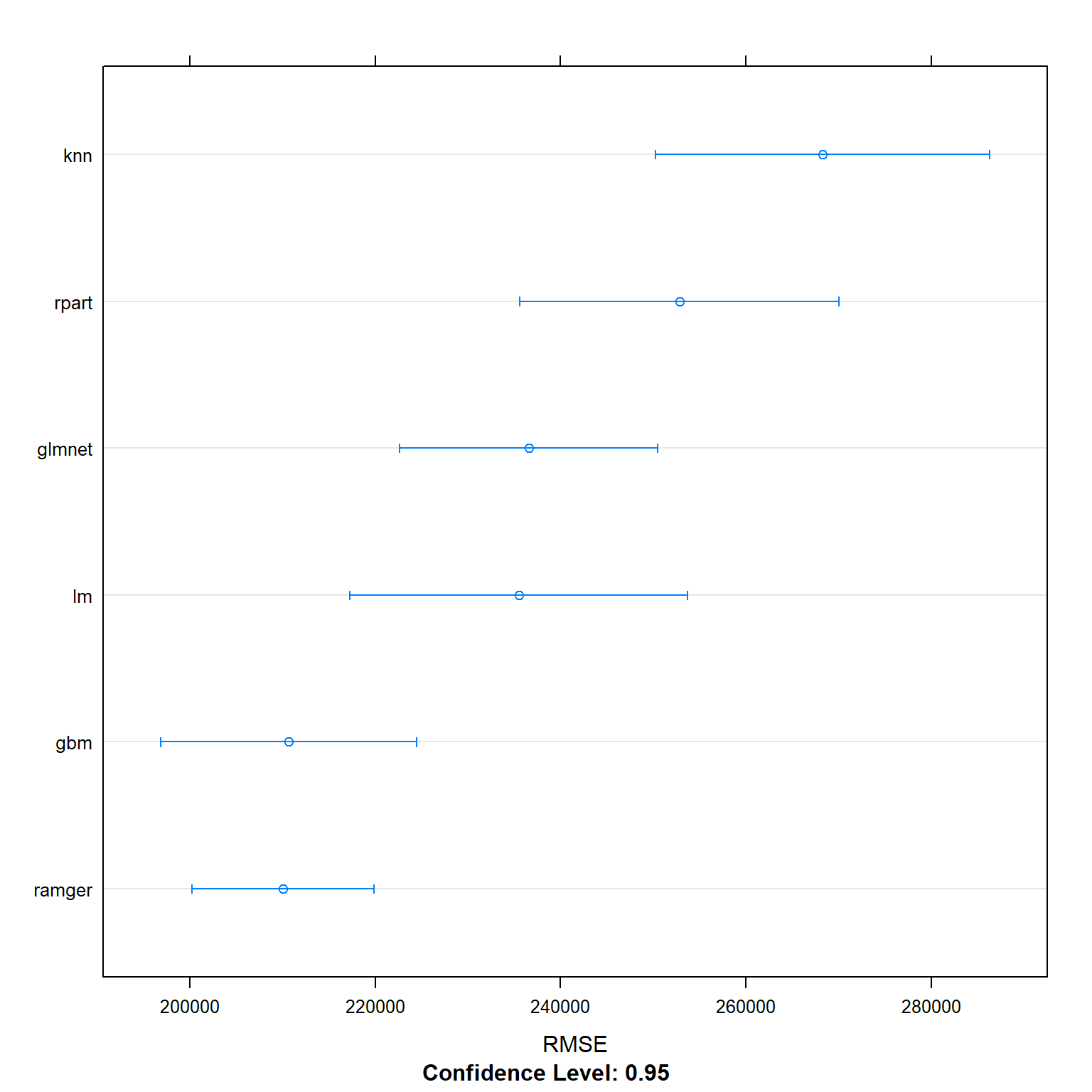
splom(resamples(multimodel), metric = "RMSE")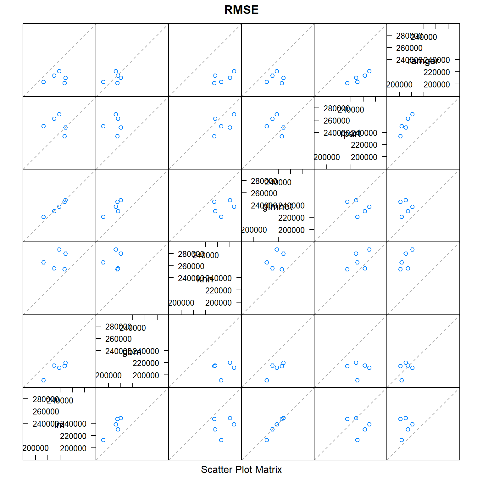
The figure below shows the correlation between the models that I stacked together. The linear regression correlated strongly with the LASSO regression, but also with gradient boost and random forest. The selection of very similar variables throughout the whole process could be a reason for this.
modelCor(resamples(multimodel))## lm gbm knn glmnet rpart ramger
## lm 1.000 0.926 0.752 0.963 0.726 0.893
## gbm 0.926 1.000 0.738 0.792 0.577 0.907
## knn 0.752 0.738 1.000 0.706 0.905 0.951
## glmnet 0.963 0.792 0.706 1.000 0.766 0.807
## rpart 0.726 0.577 0.905 0.766 1.000 0.840
## ramger 0.893 0.907 0.951 0.807 0.840 1.000Now, I run the model:
#we can now use stacking with the list of models
library(caretEnsemble)
model_list <- caretStack(multimodel,
    trControl=ctrl,
    method="lm",
    metric = "RMSE")

  summary(model_list)
##
## Call:
## lm(formula = .outcome ~ ., data = dat)
##
## Residuals:
## Min 1Q Median 3Q Max
## -3263032 -51716 1810 50039 4408661
##
## Coefficients:
## Estimate Std. Error t value Pr(>|t|)
## (Intercept) -3.36e+04 3.47e+03 -9.67 < 2e-16 ***
## lm 1.28e+00 1.16e-01 11.06 < 2e-16 ***
## gbm 3.80e-01 2.01e-02 18.95 < 2e-16 ***
## knn 1.36e-01 1.28e-02 10.59 < 2e-16 ***
## glmnet -1.13e+00 1.17e-01 -9.68 < 2e-16 ***
## rpart 6.63e-02 1.32e-02 5.01 5.4e-07 ***
## ramger 3.28e-01 2.71e-02 12.11 < 2e-16 ***
## ---
## Signif. codes: 0 '***' 0.001 '**' 0.01 '*' 0.05 '.' 0.1 ' ' 1
##
## Residual standard error: 2e+05 on 10492 degrees of freedom
## Multiple R-squared: 0.854, Adjusted R-squared: 0.854
## F-statistic: 1.02e+04 on 6 and 10492 DF, p-value: <2e-16#predict the price of each house in the test data set
#recall that the output of "train" function (knn_fit) automatically keeps the best model
all_prediction <- predict(model_list, newdata = test_data)
all_results<-data.frame(RMSE = RMSE(all_prediction, test_data$price), Rsquare = R2(all_prediction, test_data$price))
all_results## RMSE Rsquare
## 1 187360 0.866Selection of the model
To compare the performance of the different models I look at RMSE and R², the same parameters I used to optimize them. The best model is the model with the highest R² and the lowest RMSE. A high R² indicated that a high portion of overall variability in the dataset is explained by this model, while RMSE shows the error of the prediction.
data.frame(name=c("Linear Regression", "LASSO", "KNN", "Regression Tree", "Random Forest", "Gradient Boosting", "Stacked Model"),RMSE_Training= c(227300, 234251, 268281, 252842, 207808, 210764, 199600), RSquared_Training= c(0.8133, 0.8026, 0.7472, 0.7694, 0.8432
, 0.8403, 0.8541))
## name RMSE_Training RSquared_Training
## 1 Linear Regression 227300 0.813
## 2 LASSO 234251 0.803
## 3 KNN 268281 0.747
## 4 Regression Tree 252842 0.769
## 5 Random Forest 207808 0.843
## 6 Gradient Boosting 210764 0.840
## 7 Stacked Model 199600 0.854Stacking is clearly the best method, explaining 85.41% of overall variability and having the lowest error. The table shows a difference in R² and RMSE between training and testing data. While the difference is not huge, it is surprising that most models perform better in the testing data than in the training data. This is unexpected but might be caused by the seed I used when splitting the total data into training and testing. I would expect, to have a slightly different result when using another seed.
Pick investments
To select the 200 houses out of the 2,000 on the market for sale at the moment I applied my best model, the stacking model. I added the by the model predicted price to the dataset and calculated the profit margin comparing the predicted price to the asking price ((predicted price – asking price) /asking prices). Finally, I ranked the properties by the calculated profit margin and selected the top 200. These 200 properties give an average return of 69.63%. My model calculates an average return of 3.78% over the whole dataset.
numchoose=200
oos<-london_house_prices_2019_out_of_sample

#predict the value of houses
oos$predict <- predict(model_list,oos)

#Choose the ones you want to invest here

#Let's find the profit margin given our predicted price and asking price
oos_data<- oos%>%
  mutate(profitMargin=(predict-asking_price)/asking_price)%>%
  arrange(-profitMargin)

#Make sure you choose exactly 200 of them
oos_data$buy=0
oos_data[1:numchoose,]$buy=1

#let's find the actual profit

oos_data<-oos_data%>%
  mutate(actualProfit=buy*profitMargin)

#if we invest in everything
mean(oos_data$profitMargin)
## [1] 0.0378#just invest in those we chose
sum(oos_data$actualProfit)/numchoose## [1] 0.696To control, I calculate how much profit I would make on the training dataset:
##try for testing data
numchoose=200

#predict the value of houses
train_data$predict <- predict(model_list,train_data)

#Choose the ones you want to invest here
#Let's find the profit margin given our predicted price and asking price
train_data_pred<- train_data%>%
  mutate(profitMargin=(predict-price)/price)%>%
  arrange(-profitMargin)

#Make sure you choose exactly 200 of them
train_data_pred$buy=0
train_data_pred[1:numchoose,]$buy=1


#let's find the actual profit
train_data_pred<-train_data_pred%>%
  mutate(actualProfit=buy*profitMargin)

#if we invest in everything
mean(train_data_pred$actualProfit)
## [1] 0.0182#just invest in those we chose
sum(train_data_pred$actualProfit)/numchoose## [1] 0.955Conclusion
To sum up, I used available features of houses and historic data of all transactions done in London in 2019 to calculate seven different estimation engines. I used the methods linear regression, k-NN, and trees as well as the ensembled methods random forest, gradient boosting and stacking. While all of them are able to explain the difference in house prices in London at least to 75%, the best performing model, namely the stacking model, manages to explain 85.4%. This estimation engine has subsequently been used to select the 200 most promising houses to invest in, with a predicted return of 69.63%. Limitations of this project are the available information on the specific houses as well as the assumption that the asking price will not change. In addition, if I would have sufficient computing power, I would tune additional parameters of the models that I have used. Other reasonable information that could be useful is commuting time to the center especially for properties that are located far from the center, as well as distance to supermarket and other facilities. Also, the architectural style, brightness of the rooms and interior design could be significant.