SVM (Support Vector Machine): Job Attrition

Introduction
SVM (Support Vector Machine) is a supervised machine learning algorithm that is mainly used to classify data into different classes. The aim of this exercise was to predict job attrition using several individual characteristics such as distance from home, education, environment satisfaction, gender, and hourly rate and to finally predict if two specific employees would leave the job.
Preparing data
data("attrition")
# Load attrition data
set.seed(123)  # for reproducibility

df <- dplyr::mutate_if(attrition, is.ordered, factor, ordered = FALSE)

head(df)
## Age Attrition BusinessTravel DailyRate Department
## 1 41 Yes Travel_Rarely 1102 Sales
## 2 49 No Travel_Frequently 279 Research_Development
## 3 37 Yes Travel_Rarely 1373 Research_Development
## 4 33 No Travel_Frequently 1392 Research_Development
## 5 27 No Travel_Rarely 591 Research_Development
## 6 32 No Travel_Frequently 1005 Research_Development
## DistanceFromHome Education EducationField EnvironmentSatisfaction Gender
## 1 1 College Life_Sciences Medium Female
## 2 8 Below_College Life_Sciences High Male
## 3 2 College Other Very_High Male
## 4 3 Master Life_Sciences Very_High Female
## 5 2 Below_College Medical Low Male
## 6 2 College Life_Sciences Very_High Male
## HourlyRate JobInvolvement JobLevel JobRole JobSatisfaction
## 1 94 High 2 Sales_Executive Very_High
## 2 61 Medium 2 Research_Scientist Medium
## 3 92 Medium 1 Laboratory_Technician High
## 4 56 High 1 Research_Scientist High
## 5 40 High 1 Laboratory_Technician Medium
## 6 79 High 1 Laboratory_Technician Very_High
## MaritalStatus MonthlyIncome MonthlyRate NumCompaniesWorked OverTime
## 1 Single 5993 19479 8 Yes
## 2 Married 5130 24907 1 No
## 3 Single 2090 2396 6 Yes
## 4 Married 2909 23159 1 Yes
## 5 Married 3468 16632 9 No
## 6 Single 3068 11864 0 No
## PercentSalaryHike PerformanceRating RelationshipSatisfaction StockOptionLevel
## 1 11 Excellent Low 0
## 2 23 Outstanding Very_High 1
## 3 15 Excellent Medium 0
## 4 11 Excellent High 0
## 5 12 Excellent Very_High 1
## 6 13 Excellent High 0
## TotalWorkingYears TrainingTimesLastYear WorkLifeBalance YearsAtCompany
## 1 8 0 Bad 6
## 2 10 3 Better 10
## 3 7 3 Better 0
## 4 8 3 Better 8
## 5 6 3 Better 2
## 6 8 2 Good 7
## YearsInCurrentRole YearsSinceLastPromotion YearsWithCurrManager
## 1 4 0 5
## 2 7 1 7
## 3 0 0 0
## 4 7 3 0
## 5 2 2 2
## 6 7 3 6# Create training (80%) and test (20%) sets
set.seed(123) # for reproducibility
attrition_split <- initial_split(df, prop = 0.8, strata = "Attrition")
#If we want to explicitly control the sampling so that our training and test
#sets have similar y distributions, we can use stratified sampling
attrition_train <- training(attrition_split)
attrition_test <- testing(attrition_split)Radial Basis Function - SVM
#caret’s train() function with method = "svmRadialSigma" is used to get
#values of C (cost) and \sigma (related with the \gamma of Radial Basis function)
#through cross-validation
set.seed(1854)  # for reproducibility
model_svm_rbf <- train(
  Attrition ~ .,
  data = attrition_train,
  method = "svmRadial",
  preProcess = c("center", "scale"),  #x's standardized (i.e.,centered around zero with a sd of one)
  trControl = trainControl(method = "cv", number = 10),
  tuneLength = 10 #select 10 random numbers for the hypertune parameters
)

# Print results
print(model_svm_rbf$results)
## sigma C Accuracy Kappa AccuracySD KappaSD
## 1 0.009662318 0.25 0.8385702 0.0000000 0.0006647742 0.00000000
## 2 0.009662318 0.50 0.8385702 0.0000000 0.0006647742 0.00000000
## 3 0.009662318 1.00 0.8513110 0.1239377 0.0073175959 0.06778683
## 4 0.009662318 2.00 0.8657685 0.3112862 0.0163132180 0.10086539
## 5 0.009662318 4.00 0.8657685 0.3626285 0.0210030787 0.09429814
## 6 0.009662318 8.00 0.8589816 0.3852671 0.0232781466 0.09110905
## 7 0.009662318 16.00 0.8419817 0.3438177 0.0182919567 0.06346784
## 8 0.009662318 32.00 0.8326380 0.3182507 0.0177556841 0.06644716
## 9 0.009662318 64.00 0.8326380 0.3182507 0.0177556841 0.06644716
## 10 0.009662318 128.00 0.8326380 0.3182507 0.0177556841 0.06644716model_svm_rbf## Support Vector Machines with Radial Basis Function Kernel
##
## 1177 samples
## 30 predictor
## 2 classes: 'No', 'Yes'
##
## Pre-processing: centered (57), scaled (57)
## Resampling: Cross-Validated (10 fold)
## Summary of sample sizes: 1059, 1060, 1059, 1059, 1059, 1059, ...
## Resampling results across tuning parameters:
##
## C Accuracy Kappa
## 0.25 0.8385702 0.0000000
## 0.50 0.8385702 0.0000000
## 1.00 0.8513110 0.1239377
## 2.00 0.8657685 0.3112862
## 4.00 0.8657685 0.3626285
## 8.00 0.8589816 0.3852671
## 16.00 0.8419817 0.3438177
## 32.00 0.8326380 0.3182507
## 64.00 0.8326380 0.3182507
## 128.00 0.8326380 0.3182507
##
## Tuning parameter 'sigma' was held constant at a value of 0.009662318
## Accuracy was used to select the optimal model using the largest value.
## The final values used for the model were sigma = 0.009662318 and C = 4.#tune the hyperparameters with tunegrid
set.seed(1854) # for reproducibility
model_svm_rbf_2 <- train(
Attrition ~ .,
data = attrition_train,
method = "svmRadial",
preProcess = c("center", "scale"), #x's standardized (i.e.,centered around zero with a sd of one)
trControl = trainControl(method = "cv", number = 10),
tuneGrid = expand.grid(C=seq(4, 6, 1), sigma=seq(0.003,0.006,0.0005))
)
# Print results
#print(model_svm_rbf_2$results)
model_svm_rbf_2## Support Vector Machines with Radial Basis Function Kernel
##
## 1177 samples
## 30 predictor
## 2 classes: 'No', 'Yes'
##
## Pre-processing: centered (57), scaled (57)
## Resampling: Cross-Validated (10 fold)
## Summary of sample sizes: 1059, 1060, 1059, 1059, 1059, 1059, ...
## Resampling results across tuning parameters:
##
## C sigma Accuracy Kappa
## 4 0.0030 0.8674562 0.2817171
## 4 0.0035 0.8708533 0.3233907
## 4 0.0040 0.8725554 0.3387736
## 4 0.0045 0.8742721 0.3601304
## 4 0.0050 0.8751268 0.3749610
## 4 0.0055 0.8742648 0.3817300
## 4 0.0060 0.8725699 0.3766865
## 5 0.0030 0.8717080 0.3294572
## 5 0.0035 0.8768217 0.3706600
## 5 0.0040 0.8759742 0.3802197
## 5 0.0045 0.8751123 0.3836210
## 5 0.0050 0.8734246 0.3823293
## 5 0.0055 0.8734246 0.3823293
## 5 0.0060 0.8725771 0.3799746
## 6 0.0030 0.8751123 0.3658621
## 6 0.0035 0.8751195 0.3778871
## 6 0.0040 0.8751123 0.3862916
## 6 0.0045 0.8725699 0.3799100
## 6 0.0050 0.8717224 0.3775552
## 6 0.0055 0.8708822 0.3753383
## 6 0.0060 0.8717297 0.3820362
##
## Accuracy was used to select the optimal model using the largest value.
## The final values used for the model were sigma = 0.0035 and C = 5.#Plotting the results, we see that smaller values of the cost parameter
#( C≈ 2–8) provide better cross-validated accuracy scores for these
#training data:
ggplot(model_svm_rbf_2) + theme_light()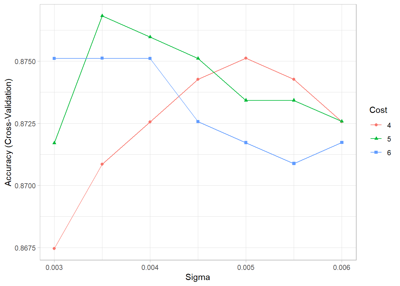
#confusion matrix on training dataset
confusionMatrix(model_svm_rbf_2)
## Cross-Validated (10 fold) Confusion Matrix
##
## (entries are percentual average cell counts across resamples)
##
## Reference
## Prediction No Yes
## No 83.2 11.6
## Yes 0.7 4.5
##
## Accuracy (average) : 0.8768## testing
#We test the model on the testing dataset
test_svm_rbf_2 = predict(model_svm_rbf_2, attrition_test)
confusionMatrix(data = test_svm_rbf_2, attrition_test$Attrition)## Confusion Matrix and Statistics
##
## Reference
## Prediction No Yes
## No 245 34
## Yes 1 13
##
## Accuracy : 0.8805
## 95% CI : (0.8378, 0.9154)
## No Information Rate : 0.8396
## P-Value [Acc > NIR] : 0.03008
##
## Kappa : 0.3806
##
## Mcnemar's Test P-Value : 6.338e-08
##
## Sensitivity : 0.9959
## Specificity : 0.2766
## Pos Pred Value : 0.8781
## Neg Pred Value : 0.9286
## Prevalence : 0.8396
## Detection Rate : 0.8362
## Detection Prevalence : 0.9522
## Balanced Accuracy : 0.6363
##
## 'Positive' Class : No
## After loading the dataset “attrition”, I transform the data to the format of an SVM package (outcome as factor). Then, I set a seed for reproducibility and split the data into a training & testing dataset, explicitly controlling the sampling so that both have a similar distribution of y. To classify the employees based in the given features into “yes” and “no”, we use the radial basis function kernel. This function transforms the data points to generate new features by measuring the distance between all other points to a specific dot centre. Doing so it projects all points into an “infinite” higher dimensional space where the data becomes linearly separable. Before running the model with the method “svmRadial” of caret’s train() function, I again set a seed. I could optimize the model using different metrics such as accuracy and ROC. Here, I use “accuracy” to select the best model. When running the model, I standardize the data by centring and scaling the data. I use cross-sampling (10-fold) as resampling method and tune the value C & γ. TuneLength = 10 takes 10 random values of C & γ and gives the best output amongst these randomly chosen numbers. Subsequently, I further tune the parameters by using tuneGrid around the output of tuneLength. Optimizing “accuracy” the final model I select has sigma = 0.0035, C = 5, and reaches an accuracy of 87.68% with a sensitivity of 99.59% and a specificity of 27.66% . Now, I predict the classes on the testing dataset and compare the predicted classification with the labels of the dataset. On the testing dataset, this model reaches an accuracy of 88.05%. (Sensitivity: 99.59%, Specificity: 27.66%, Balanced Accuracy: 63.63%.)
##2 Linear kernel function
#
set.seed(1854)  # for reproducibility
# Tell SVM that the kernel is linear, the tune-in parameter cost is 5, and scale equals true.

##2 linear with caret package
set.seed(1854)  # for reproducibility
model_svm_linear_2 <- train(
  Attrition ~ .,
  data = attrition_train,
  method = "svmLinear",
  preProcess = c("center", "scale"),  #x's standardized (i.e.,centered around zero with a sd of one)
  trControl = trainControl(method = "cv", number = 10),
  tuneGrid = expand.grid(C=5)
)

#print results
print(model_svm_linear_2$results)
## C Accuracy Kappa AccuracySD KappaSD
## 1 5 0.870042 0.4252287 0.02902589 0.1192711## testing
#We test the model on the testing dataset
test_svm_linear_2 = predict(model_svm_linear_2, attrition_test)
confusionMatrix(data = test_svm_linear_2, attrition_test$Attrition)## Confusion Matrix and Statistics
##
## Reference
## Prediction No Yes
## No 241 23
## Yes 5 24
##
## Accuracy : 0.9044
## 95% CI : (0.8648, 0.9356)
## No Information Rate : 0.8396
## P-Value [Acc > NIR] : 0.0009129
##
## Kappa : 0.5802
##
## Mcnemar's Test P-Value : 0.0013149
##
## Sensitivity : 0.9797
## Specificity : 0.5106
## Pos Pred Value : 0.9129
## Neg Pred Value : 0.8276
## Prevalence : 0.8396
## Detection Rate : 0.8225
## Detection Prevalence : 0.9010
## Balanced Accuracy : 0.7452
##
## 'Positive' Class : No
## Comparison of SVM RBF and SVM with Linear kernel function (c=5)
As second model I use the SVM model with the linear kernel function. Here, I use the same cost factor that I determined in the first model (cost = 5). A linear SVM is a parametric model, and is less expensive to train and predict than a RBF kernel SVM model. Besides being more computational expensive, the latter it much easier to overfit being a complex model with many hyperparameters.
Here, this model gives an accuracy of 87.00%, what is slightly lower than the accuracy of the SVM EBF model, with an accuracy if 87.68%. The out of sample testing performs better though, with an accuracy of 90.44% (compared to an accuracy of 88.05%).
##3 Logistic Regression
model_logistic <- glm(Attrition~BusinessTravel + DistanceFromHome + EnvironmentSatisfaction +
                      Gender+ JobInvolvement + JobRole  + MaritalStatus+
                      NumCompaniesWorked + OverTime + RelationshipSatisfaction+ TotalWorkingYears+
                      TrainingTimesLastYear+ WorkLifeBalance+ YearsInCurrentRole + YearsSinceLastPromotion,
                    family="binomial", attrition_train)

summary(model_logistic)
##
## Call:
## glm(formula = Attrition ~ BusinessTravel + DistanceFromHome +
## EnvironmentSatisfaction + Gender + JobInvolvement + JobRole +
## MaritalStatus + NumCompaniesWorked + OverTime + RelationshipSatisfaction +
## TotalWorkingYears + TrainingTimesLastYear + WorkLifeBalance +
## YearsInCurrentRole + YearsSinceLastPromotion, family = "binomial",
## data = attrition_train)
##
## Deviance Residuals:
## Min 1Q Median 3Q Max
## -1.8768 -0.4944 -0.2749 -0.1033 3.9483
##
## Coefficients:
## Estimate Std. Error z value Pr(>|z|)
## (Intercept) -0.90029 0.83791 -1.074 0.282621
## BusinessTravelTravel_Frequently 1.60242 0.42480 3.772 0.000162 ***
## BusinessTravelTravel_Rarely 0.95694 0.39118 2.446 0.014433 *
## DistanceFromHome 0.04324 0.01164 3.714 0.000204 ***
## EnvironmentSatisfactionMedium -1.11996 0.30199 -3.709 0.000208 ***
## EnvironmentSatisfactionHigh -1.01384 0.26613 -3.810 0.000139 ***
## EnvironmentSatisfactionVery_High -1.34486 0.27659 -4.862 1.16e-06 ***
## GenderMale 0.40817 0.20008 2.040 0.041352 *
## JobInvolvementMedium -0.75783 0.38054 -1.991 0.046428 *
## JobInvolvementHigh -1.24222 0.36043 -3.447 0.000568 ***
## JobInvolvementVery_High -1.68965 0.49486 -3.414 0.000639 ***
## JobRoleHuman_Resources 2.04238 0.59622 3.426 0.000614 ***
## JobRoleLaboratory_Technician 1.54114 0.48297 3.191 0.001418 **
## JobRoleManager 0.48627 0.73624 0.660 0.508944
## JobRoleManufacturing_Director 0.34080 0.60355 0.565 0.572306
## JobRoleResearch_Director -1.20518 1.16715 -1.033 0.301799
## JobRoleResearch_Scientist 0.60884 0.48803 1.248 0.212201
## JobRoleSales_Executive 1.08881 0.47868 2.275 0.022928 *
## JobRoleSales_Representative 2.16183 0.55651 3.885 0.000102 ***
## MaritalStatusMarried 0.22081 0.27805 0.794 0.427125
## MaritalStatusSingle 1.22718 0.28184 4.354 1.34e-05 ***
## NumCompaniesWorked 0.15355 0.04087 3.757 0.000172 ***
## OverTimeYes 2.05669 0.21338 9.639 < 2e-16 ***
## RelationshipSatisfactionMedium -0.80170 0.30498 -2.629 0.008571 **
## RelationshipSatisfactionHigh -0.83069 0.27632 -3.006 0.002645 **
## RelationshipSatisfactionVery_High -0.92268 0.28118 -3.281 0.001033 **
## TotalWorkingYears -0.09092 0.02384 -3.814 0.000137 ***
## TrainingTimesLastYear -0.19553 0.08021 -2.438 0.014786 *
## WorkLifeBalanceGood -1.15480 0.38988 -2.962 0.003057 **
## WorkLifeBalanceBetter -1.44181 0.36179 -3.985 6.74e-05 ***
## WorkLifeBalanceBest -0.84796 0.44227 -1.917 0.055204 .
## YearsInCurrentRole -0.11146 0.04329 -2.575 0.010035 *
## YearsSinceLastPromotion 0.16997 0.04299 3.954 7.69e-05 ***
## ---
## Signif. codes: 0 '***' 0.001 '**' 0.01 '*' 0.05 '.' 0.1 ' ' 1
##
## (Dispersion parameter for binomial family taken to be 1)
##
## Null deviance: 1040.54 on 1176 degrees of freedom
## Residual deviance: 717.82 on 1144 degrees of freedom
## AIC: 783.82
##
## Number of Fisher Scoring iterations: 7#to get accuracy of the training data
probabilities_attrition_train <- model_logistic %>% predict(attrition_train, type = "response")
predicted.classes_train <- ifelse(probabilities_attrition_train > 0.5, "Yes", "No")
mean(predicted.classes_train == attrition_train$Attrition)## [1] 0.8810535probabilities_attrition <- model_logistic %>% predict(attrition_test, type = "response")
predicted.classes <- as.factor(ifelse(probabilities_attrition > 0.5, "Yes", "No"))
#Accuracy: The model accuracy is measured as the proportion of observations that have been correctly classified.
#Inversely, the classification error is defined as the proportion of observations that have been misclassified.
#Proportion of correctly classified observations:
mean(predicted.classes == attrition_test$Attrition)## [1] 0.887372confusionMatrix(data = predicted.classes, attrition_test$Attrition)## Confusion Matrix and Statistics
##
## Reference
## Prediction No Yes
## No 236 23
## Yes 10 24
##
## Accuracy : 0.8874
## 95% CI : (0.8455, 0.9212)
## No Information Rate : 0.8396
## P-Value [Acc > NIR] : 0.01302
##
## Kappa : 0.5292
##
## Mcnemar's Test P-Value : 0.03671
##
## Sensitivity : 0.9593
## Specificity : 0.5106
## Pos Pred Value : 0.9112
## Neg Pred Value : 0.7059
## Prevalence : 0.8396
## Detection Rate : 0.8055
## Detection Prevalence : 0.8840
## Balanced Accuracy : 0.7350
##
## 'Positive' Class : No
## Now, I create a model using a logistic regression and compare it with the SVM classifier. I select the variables that are significant for the logistic regression such as business travel, distance from home, and environment satisfaction. The logistic regression gives me only a probability for attrition; therefore, I need to set a cut-off value. I set the cut-off value at 50% (every value > 50% = “Yes”). The accuracy for this model is 88.11% which is better than both SVM models. Out of sample accuracy amounts to 88.74%.
##KNN
set.seed(1234) #I will use cross validation. To be able to replicate the results I set the seed to a fixed number

# Below I use 'train' function from caret library.
# 'preProcess': I use this option to center and scale the data
# 'method' is knn
# default 'metric' is accuracy

model_knn <- train(Attrition~., data=attrition_train,
                 method = "knn",
                 trControl = trainControl("cv", number = 10), #use cross validation with 10 data points
                 tuneLength = 10, #number of parameter values train function will try
                 preProcess = c("center", "scale"))  #center and scale the data in k-nn this is pretty important

model_knn
## k-Nearest Neighbors
##
## 1177 samples
## 30 predictor
## 2 classes: 'No', 'Yes'
##
## Pre-processing: centered (57), scaled (57)
## Resampling: Cross-Validated (10 fold)
## Summary of sample sizes: 1059, 1060, 1059, 1059, 1059, 1060, ...
## Resampling results across tuning parameters:
##
## k Accuracy Kappa
## 5 0.8385702 0.12216802
## 7 0.8411415 0.11075104
## 9 0.8428147 0.08514906
## 11 0.8436694 0.08242729
## 13 0.8445386 0.07600373
## 15 0.8445241 0.07107637
## 17 0.8428220 0.05459990
## 19 0.8436694 0.05666231
## 21 0.8436622 0.05001399
## 23 0.8411198 0.02556860
##
## Accuracy was used to select the optimal model using the largest value.
## The final value used for the model was k = 13.plot(model_knn) #we can plot the results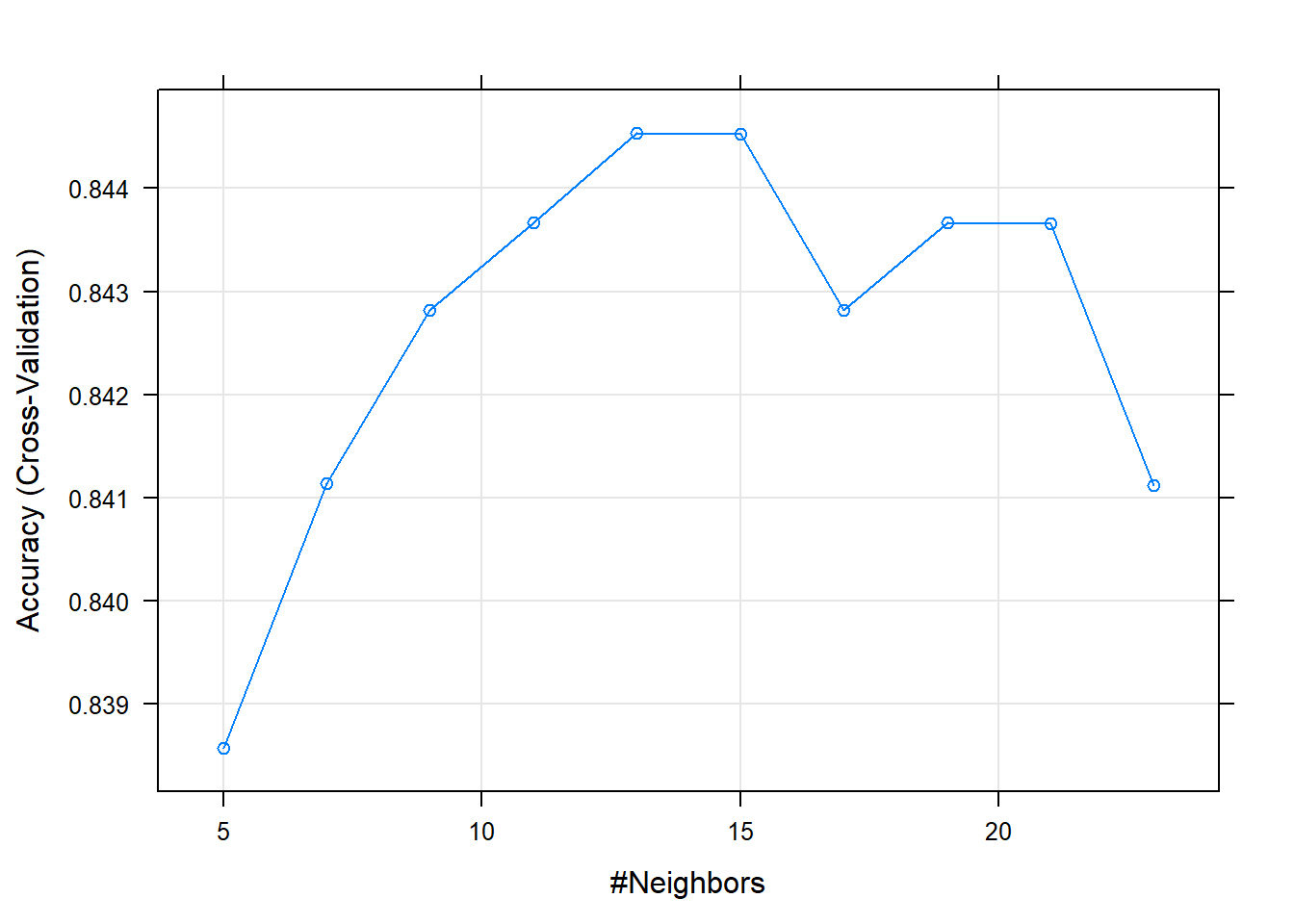
# very low accuracy compared to others - I don't continue to tune with grid.

## testing
#We test the model on the testing dataset
test_knn = predict(model_knn, attrition_test)
confusionMatrix(data = test_knn, attrition_test$Attrition)
## Confusion Matrix and Statistics
##
## Reference
## Prediction No Yes
## No 246 46
## Yes 0 1
##
## Accuracy : 0.843
## 95% CI : (0.7962, 0.8827)
## No Information Rate : 0.8396
## P-Value [Acc > NIR] : 0.4754
##
## Kappa : 0.0352
##
## Mcnemar's Test P-Value : 3.247e-11
##
## Sensitivity : 1.00000
## Specificity : 0.02128
## Pos Pred Value : 0.84247
## Neg Pred Value : 1.00000
## Prevalence : 0.83959
## Detection Rate : 0.83959
## Detection Prevalence : 0.99659
## Balanced Accuracy : 0.51064
##
## 'Positive' Class : No
## KNN Model As fourth model I use the k-Nearest Neighbours (k-NN) model. It predicts a value based on a datapoint’s k nearest neighbours. This means, that the probability of attrition is predicted based on the k most similar properties in the training dataset. Amongst the 10 randomly selected k, the model with k= 13 performs best, with an accuracy of 84.45%.
Comparing the models
Comparing the four models based on accuracy, all models other than KNN, perform similarly well. KNN is the weakest model. All four models are not overfitted, having the out of sample accuracy similar or even higher to the accuracy on the training data.
Accuracy (training data) Accuracy (testing data)SVM RBF 0.8768 0.8805 SVM Linear 0.8700 0.9044 Logistic regression 0.8811 0.8874 KNN 0.8445 0.843
Below you find listed some differences between SVM and Logistic Regression:
SVM (RBF)
- Optimizes the margin that separates the two classes
- For unstructured and semi-structured data like text and images
- Less vulnerable to overfitting
- Based on geometrical properties
Logistic Regression - Can have different decision boundaries with different weights to predict - Works with already defined independent variables - Based on statistical approach - More vulnerable to overfitting
In general, with a high number of features and a small training set, it is better to use a logistic regression or SVM with linear kernel. Logistic regression and SVM with a linear kernel perform usually similarly but depending on the features, one could be more efficient than the other. In this case, I would recommend using the logistic regression as it is a less complex model, does not over-fit, is not computational heavy and performs as well as the other models.
Applying the best model
#load dataset
library(readr)
two_employees <- read_csv("data/two_employees.csv")
## Parsed with column specification:
## cols(
## .default = col_double(),
## Employee = col_character(),
## BusinessTravel = col_character(),
## Department = col_character(),
## Education = col_character(),
## EducationField = col_character(),
## EnvironmentSatisfaction = col_character(),
## Gender = col_character(),
## JobInvolvement = col_character(),
## JobRole = col_character(),
## JobSatisfaction = col_character(),
## MaritalStatus = col_character(),
## OverTime = col_character(),
## PerformanceRating = col_character(),
## RelationshipSatisfaction = col_character(),
## WorkLifeBalance = col_character()
## )## See spec(...) for full column specifications.two_employees <- two_employees %>%
mutate_if(is.ordered, factor, ordered = FALSE)
head(two_employees)## # A tibble: 2 x 31
## Employee Age BusinessTravel DailyRate Department DistanceFromHome Education
## <chr> <dbl> <chr> <dbl> <chr> <dbl> <chr>
## 1 A 48 Travel_Rarely 1202 Sales 8 College
## 2 B 38 Travel_Rarely 1218 Sales 9 Master
## # ... with 24 more variables: EducationField <chr>,
## # EnvironmentSatisfaction <chr>, Gender <chr>, HourlyRate <dbl>,
## # JobInvolvement <chr>, JobLevel <dbl>, JobRole <chr>, JobSatisfaction <chr>,
## # MaritalStatus <chr>, MonthlyIncome <dbl>, MonthlyRate <dbl>,
## # NumCompaniesWorked <dbl>, OverTime <chr>, PercentSalaryHike <dbl>,
## # PerformanceRating <chr>, RelationshipSatisfaction <chr>,
## # StockOptionLevel <dbl>, TotalWorkingYears <dbl>,
## # TrainingTimesLastYear <dbl>, WorkLifeBalance <chr>, YearsAtCompany <dbl>,
## # YearsInCurrentRole <dbl>, YearsSinceLastPromotion <dbl>,
## # YearsWithCurrManager <dbl>#predict attrition
probabilities_attrition_two_employees <- model_logistic %>% predict(two_employees, type = "response")
predicted.classes_two_employees <- as.factor(ifelse(probabilities_attrition_two_employees > 0.5, "Yes", "No"))
predicted.classes_two_employees## 1 2
## Yes No
## Levels: No YesIn this exercise, I predict with the logistic regression if the two employees given their characteristics would be likely to leave their job.
I use the logistic regression to classify the two employees: According to the logistical model, employee A is likely to leave the job, while employee B not. Given the characteristics of employee A and B, without this prediction with the model I would have rather guessed that employee B could be likely to leave the job (given the los job satisfaction). But it seems that other characteristics have a higher impact on the likeliness of job attrition. To keep the employee A, probably a better life work balance, percentage salary hike, relationship satisfaction and no over time would be needed.